topmodels

Worm Plots for Quantile Residuals

Description

Visualize goodness of fit of regression models by worm plots using quantile residuals. If plot = TRUE, the resulting object of class “wormplot” is plotted by plot.qqrplot or autoplot.qqrplot before it is returned, depending on whether the package ggplot2 is loaded.

Usage

wormplot(object, ...)

## Default S3 method:
wormplot(
  object,
  newdata = NULL,
  plot = TRUE,
  class = NULL,
  detrend = TRUE,
  scale = c("normal", "uniform"),
  nsim = 1L,
  delta = NULL,
  confint = TRUE,
  simint = TRUE,
  simint_level = 0.95,
  simint_nrep = 250,
  single_graph = FALSE,
  xlab = "Theoretical quantiles",
  ylab = "Deviation",
  main = NULL,
  ...
)

Arguments

`object`	an object from which probability integral transforms can be extracted using the generic function `procast`.
`newdata`	optionally, a data frame in which to look for variables with which to predict. If omitted, the original observations are used.
`plot`	Should the `plot` or `autoplot` method be called to draw the computed Q-Q plot? Either set `plot` expicitly to `“base”` vs. `“ggplot2”` to choose the type of plot, or for a logical `plot` argument it’s chosen conditional if the package `ggplot2` is loaded.
`class`	Should the invisible return value be either a `data.frame` or a `tibble`. Either set `class` expicitly to `“data.frame”` vs. `“tibble”`, or for `NULL` it’s chosen automatically conditional if the package `tibble` is loaded.
`detrend`	logical. Should the qqrplot be detrended, i.e, plotted as a ‘wormplot()’?
`scale`	On which scale should the quantile residuals be shown: on the probability scale (`“uniform”`) or on the normal scale (`“normal”`).
`nsim`, `delta`	arguments passed to `proresiduals`.
`confint`	logical or character string describing the type for plotting ‘c("polygon", "line")’. If not set to ‘FALSE’, the pointwise confidence interval of the (randomized) quantile residuals are visualized.
`simint`	logical. In case of discrete distributions, should the simulation (confidence) interval due to the randomization be visualized?
`simint_level`	numeric. The confidence level required for calculating the simulation (confidence) interval due to the randomization.
`simint_nrep`	numeric. The repetition number of simulated quantiles for calculating the simulation (confidence) interval due to the randomization.
`single_graph`	logical. Should all computed extended reliability diagrams be plotted in a single graph?
`xlab`, `ylab`, `main`, `…`	graphical parameters passed to `plot.qqrplot` or `autoplot.qqrplot`.

Details

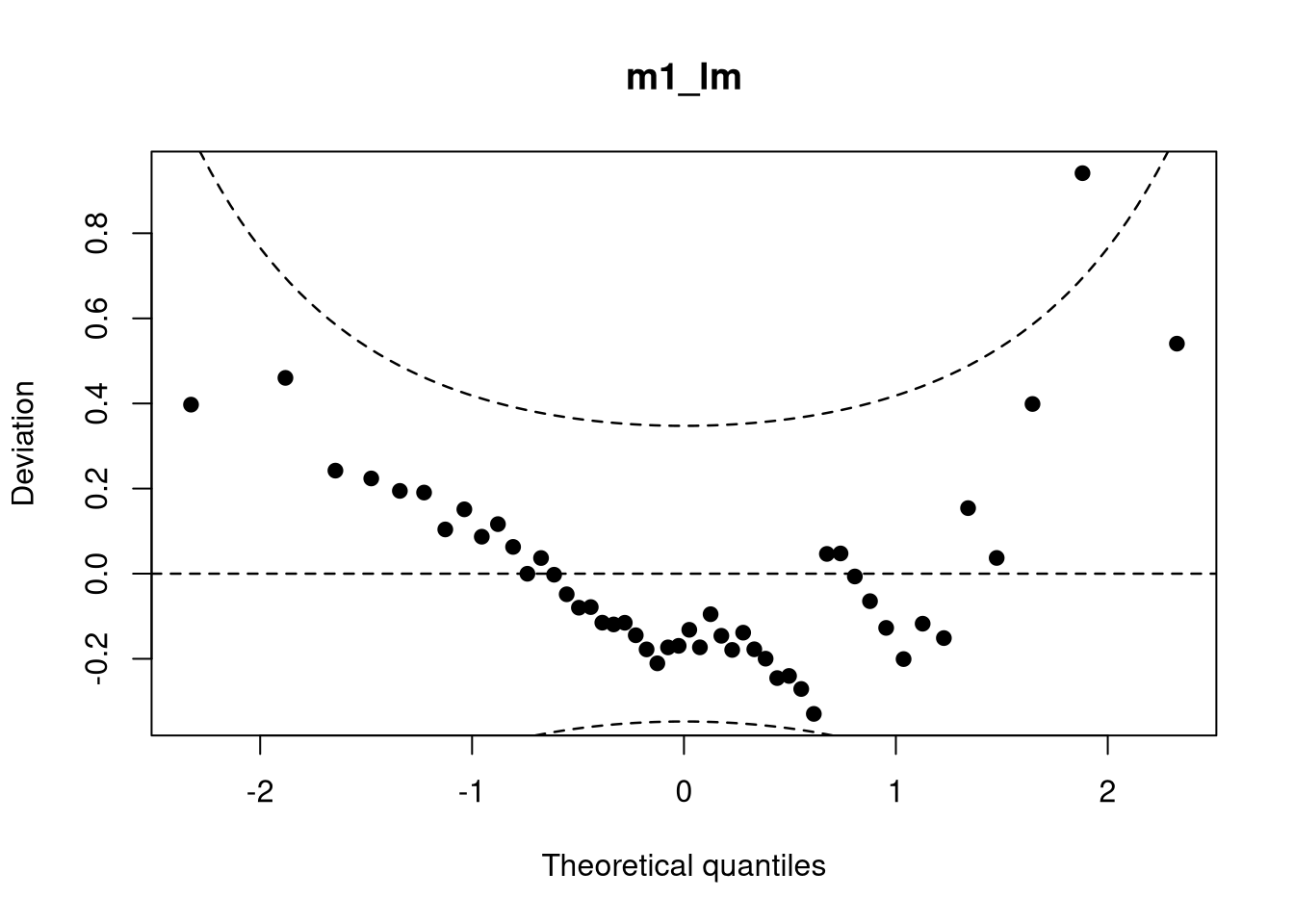
Worm plots (de-trended Q-Q plots) draw deviations of quantile residuals (by default: transformed to standard normal scale) and theoretical quantiles from the same distribution against the same theoretical quantiles. For computation, wormplot leverages the function proresiduals employing the procast.

Additional options are offered for models with discrete responses where randomization of quantiles is needed.

In addition to the plot and autoplot method for wormplot objects, it is also possible to combine two (or more) worm plots by c/rbind, which creates a set of worm plots that can then be plotted in one go.

Value

An object of class “qqrplot” inheriting from “data.frame” or “tibble” conditional on the argument class with the following variables:

`x`	theoretical quantiles,
`y`	deviations between theoretical and empirical quantiles.

In case of randomized residuals, nsim different x and y values, and lower and upper confidence interval bounds (x_rg_lwr, y_rg_lwr, x_rg_upr, y_rg_upr) can optionally be returned. Additionally, xlab, ylab, main, and simint_level, as well as the the (scale) and wether a detrended Q-Q residuals plot was computed are stored as attributes.

References

van Buuren S and Fredriks M (2001). “Worm plot: simple diagnostic device for modelling growth reference curves”. Statistics in Medicine, 20, 1259–1277. doi:10.1002/sim.746

Examples

library("topmodels")


## speed and stopping distances of cars
m1_lm <- lm(dist ~ speed, data = cars)

## compute and plot wormplot
wormplot(m1_lm)

#-------------------------------------------------------------------------------
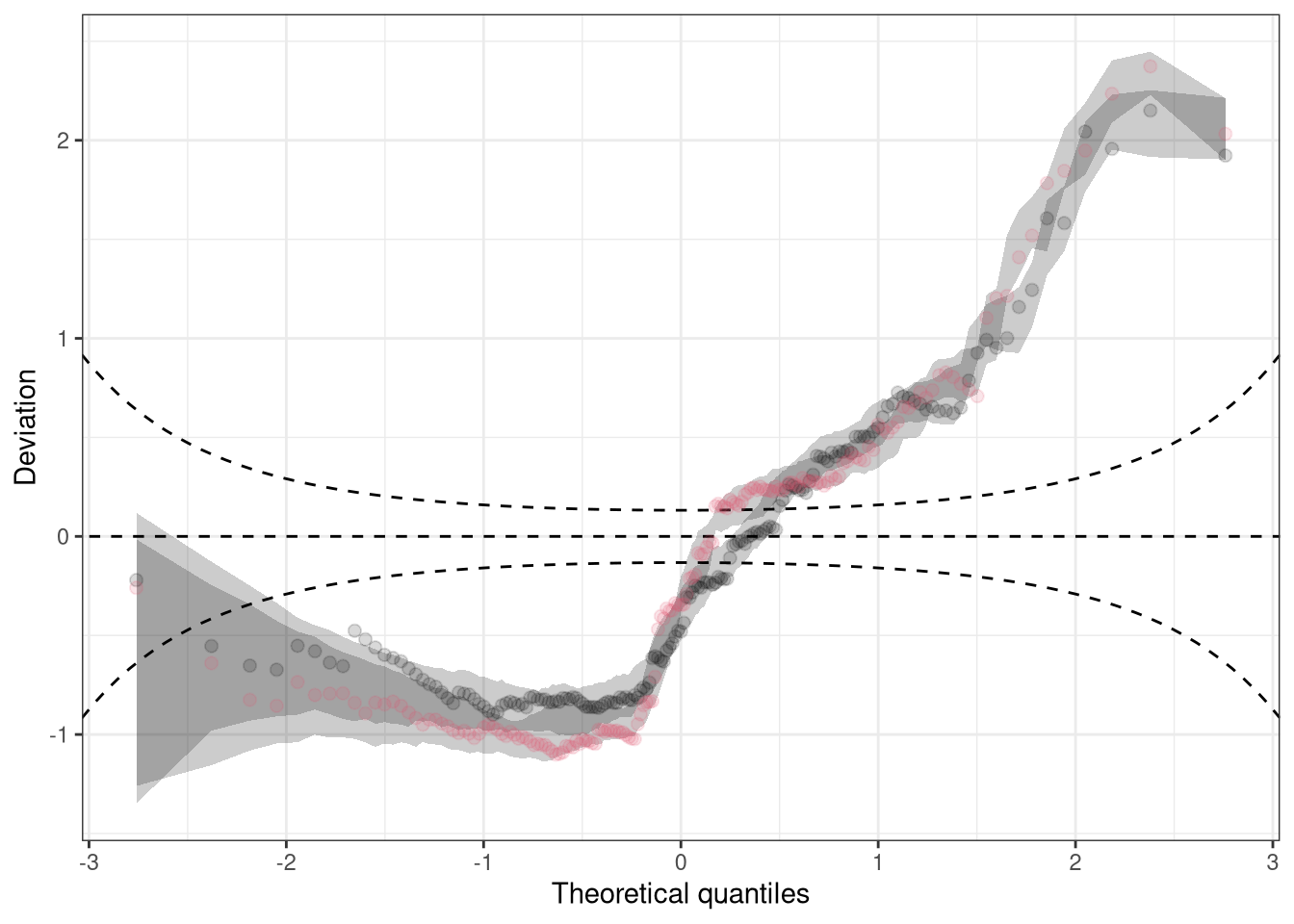
## determinants for male satellites to nesting horseshoe crabs
data("CrabSatellites", package = "countreg")

## linear poisson model
m1_pois <- glm(satellites ~ width + color, data = CrabSatellites, family = poisson)
m2_pois <- glm(satellites ~ color, data = CrabSatellites, family = poisson)

## compute and plot wormplot as base graphic
w1 <- wormplot(m1_pois, plot = FALSE)
w2 <- wormplot(m2_pois, plot = FALSE)

## plot combined wormplot as "ggplot2" graphic
ggplot2::autoplot(c(w1, w2), single_graph = TRUE, col = c(1, 2), fill = c(1, 2))