S3 Methods for Plotting PIT Histograms

Description

Generic plotting functions for probability integral transform (PIT) histograms of the class “pithist” computed by link{pithist}.

Usage

## S3 method for class 'pithist'
plot(
  x,
  single_graph = FALSE,
  style = NULL,
  freq = NULL,
  expected = TRUE,
  confint = NULL,
  confint_level = 0.95,
  confint_type = c("exact", "approximation"),
  simint = NULL,
  xlim = c(NA, NA),
  ylim = c(0, NA),
  xlab = NULL,
  ylab = NULL,
  main = NULL,
  axes = TRUE,
  box = TRUE,
  col = "black",
  border = "black",
  lwd = NULL,
  lty = 1,
  alpha_min = 0.2,
  expected_col = NULL,
  expected_lty = NULL,
  expected_lwd = 1.75,
  confint_col = NULL,
  confint_lty = 2,
  confint_lwd = 1.75,
  confint_alpha = NULL,
  simint_col = "black",
  simint_lty = 1,
  simint_lwd = 1.75,
  ...
)

## S3 method for class 'pithist'
lines(
  x,
  freq = NULL,
  expected = FALSE,
  confint = FALSE,
  confint_level = 0.95,
  confint_type = c("exact", "approximation"),
  simint = FALSE,
  col = "black",
  lwd = 2,
  lty = 1,
  expected_col = "black",
  expected_lty = 2,
  expected_lwd = 1.75,
  confint_col = "black",
  confint_lty = 1,
  confint_lwd = 1.75,
  confint_alpha = 1,
  simint_col = "black",
  simint_lty = 1,
  simint_lwd = 1.75,
  ...
)

## S3 method for class 'pithist'
autoplot(
  object,
  single_graph = FALSE,
  style = NULL,
  freq = NULL,
  expected = NULL,
  confint = NULL,
  confint_level = 0.95,
  confint_type = c("exact", "approximation"),
  simint = NULL,
  xlim = c(NA, NA),
  ylim = c(0, NA),
  xlab = NULL,
  ylab = NULL,
  main = NULL,
  legend = FALSE,
  theme = NULL,
  colour = NULL,
  fill = NULL,
  size = NULL,
  linetype = NULL,
  alpha = NULL,
  expected_colour = NULL,
  expected_size = 0.75,
  expected_linetype = NULL,
  expected_alpha = NA,
  confint_colour = NULL,
  confint_fill = NULL,
  confint_size = 0.75,
  confint_linetype = NULL,
  confint_alpha = NULL,
  simint_colour = "black",
  simint_size = 0.5,
  simint_linetype = 1,
  simint_alpha = NA,
  ...
)

Arguments

single_graph	logical. Should all computed extended reliability diagrams be plotted in a single graph? If yes, style must be set to “line”.
style	NULL or character specifying the style of pithist. For style = “bar” a traditional PIT hisogram is drawn, for style = “line” solely the upper border line is plotted. single_graph = TRUE always results in a combined line-style PIT histogram.
freq	NULL or logical. TRUE will enforce the PIT to be represented by frequencies (counts) while FALSE will enforce densities.
expected	logical. Should the expected values be plotted as reference?
confint	NULL or logical. Should confident intervals be drawn? Either logical or as
confint_level	numeric in [0, 1]. The confidence level to be shown.
confint_type	character. Which type of confidence interval should be plotted: ‘"exact"’ or ‘"approximation"’. According to Agresti and Coull (1998), for interval estimation of binomial proportions an approximation can be better than exact.
simint	NULL or logical. In case of discrete distributions, should the simulation (confidence) interval due to the randomization be visualized? character string defining one of ‘"polygon"’, ‘"line"’ or ‘"none"’. If freq = NULL it is taken from the object.
xlim, ylim, xlab, ylab, main, axes, box	graphical parameters.
col, border, lwd, lty, alpha_min	graphical parameters for the main part of the base plot.
simint_col, simint_lty, simint_lwd, confint_col, confint_lty, confint_lwd, confint_alpha, expected_col, expected_lty, expected_lwd	Further graphical parameters for the ‘confint’ and ‘simint’ line/polygon in the base plot.
…	further graphical parameters passed to the plotting function.
object, x	an object of class pithist.
legend	logical. Should a legend be added in the ggplot2 style graphic?
theme	Which ‘ggplot2’ theme should be used. If not set, theme_bw is employed.
colour, fill, size, linetype, alpha	graphical parameters for the histogram style part in the autoplot.
simint_colour, simint_size, simint_linetype, simint_alpha, confint_colour, confint_fill, confint_size, confint_linetype, expected_colour, expected_size, expected_linetype, expected_alpha	Further graphical parameters for the ‘confint’ and ‘simint’ line/polygon using autoplot.

Details

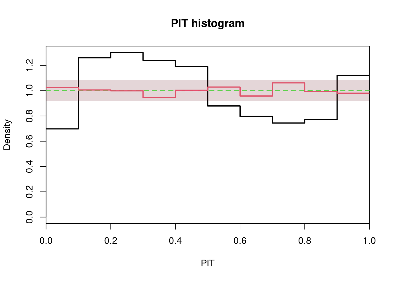
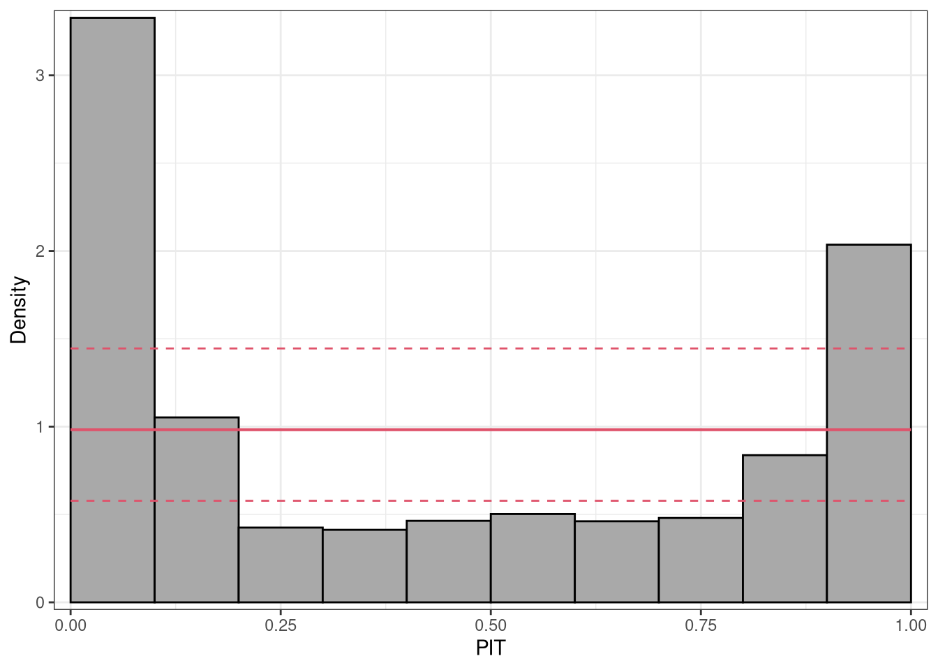
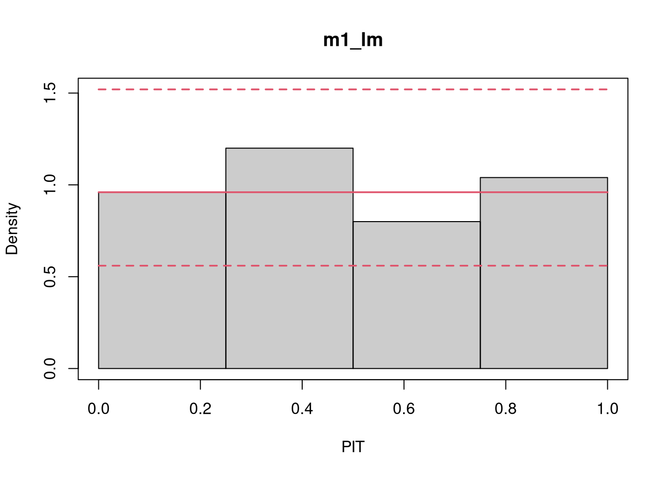
PIT histograms graphically evaluate the probability integral transform (PIT), i.e., the value that the predictive CDF attains at the observation, with a uniform distribution. For a well calibrated model fit, the observation will be drawn from the predictive distribution and the PIT will have a standard uniform distribution.

PIT histograms can be rendered as ggplot2 or base R graphics by using the generics autoplot or plot. For a single base R graphically panel, lines adds an additional PIT histogram.

References

Agresti A, Coull AB (1998). “Approximate is Better than “Exact” for Interval Estimation of Binomial Proportions.” The American Statistician, 52(2), 119–126. doi:10.1080/00031305.1998.10480550

Czado C, Gneiting T, Held L (2009). “Predictive Model Assessment for Count Data.” Biometrics, 65(4), 1254–1261. doi:10.2307/2981683

Dawid AP (1984). “Present Position and Potential Developments: Some Personal Views: Statistical Theory: The Prequential Approach”, Journal of the Royal Statistical Society: Series A (General), 147(2), 278–292. doi:10.2307/2981683

Diebold FX, Gunther TA, Tay AS (1998). “Evaluating Density Forecasts with Applications to Financial Risk Management”. International Economic Review, 39(4), 863–883. doi:10.2307/2527342

Gneiting T, Balabdaoui F, Raftery AE (2007). “Probabilistic Forecasts, Calibration and Sharpness”. Journal of the Royal Statistical Society: Series B (Methodological). 69(2), 243–268. doi:10.1111/j.1467-9868.2007.00587.x

See Also

pithist, procast, hist

Examples

library("topmodels")


## speed and stopping distances of cars
m1_lm <- lm(dist ~ speed, data = cars)

## compute and plot pithist
pithist(m1_lm)

## customize colors and style
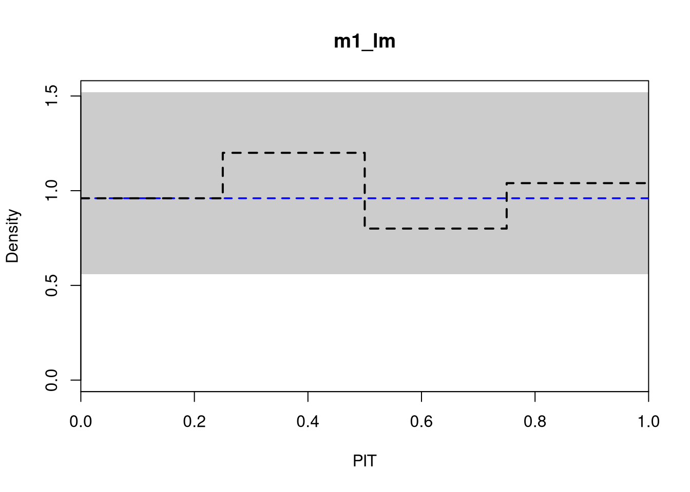
pithist(m1_lm, expected_col = "blue", lty = 2, pch = 20, style = "line")

## add separate model
if (require("crch", quietly = TRUE)) {
  m1_crch <- crch(dist ~ speed | speed, data = cars)
  #lines(pithist(m1_crch, plot = FALSE), col = 2, lty = 2, confint_col = 2) #FIXME
}

#-------------------------------------------------------------------------------
if (require("crch")) {

  ## precipitation observations and forecasts for Innsbruck
  data("RainIbk", package = "crch")
  RainIbk <- sqrt(RainIbk)
  RainIbk$ensmean <- apply(RainIbk[, grep("^rainfc", names(RainIbk))], 1, mean)
  RainIbk$enssd <- apply(RainIbk[, grep("^rainfc", names(RainIbk))], 1, sd)
  RainIbk <- subset(RainIbk, enssd > 0)

  ## linear model w/ constant variance estimation
  m2_lm <- lm(rain ~ ensmean, data = RainIbk)

  ## logistic censored model
  m2_crch <- crch(rain ~ ensmean | log(enssd), data = RainIbk, left = 0, dist = "logistic")

  ## compute pithists
  pit2_lm <- pithist(m2_lm, plot = FALSE)
  pit2_crch <- pithist(m2_crch, plot = FALSE)

  ## plot in single graph with style "line"
  plot(c(pit2_lm, pit2_crch),
    col = c(1, 2), confint_col = c(1, 2), expected_col = 3,
    style = "line", single_graph = TRUE
  )
}

#-------------------------------------------------------------------------------
## determinants for male satellites to nesting horseshoe crabs
data("CrabSatellites", package = "countreg")

## linear poisson model
m3_pois <- glm(satellites ~ width + color, data = CrabSatellites, family = poisson)

## compute and plot pithist as "ggplot2" graphic
pithist(m3_pois, plot = "ggplot2")