topmodels

Reliagram (Extended Reliability Diagram)

Description

Reliagram (extended reliability diagram) assess the reliability of a fitted probabilistic distributional forecast for a binary event. If plot = TRUE, the resulting object of class “reliagram” is plotted by plot.reliagram or autoplot.reliagram before it is returned, depending on whether the package ggplot2 is loaded.

Usage

reliagram(object, ...)

## Default S3 method:
reliagram(
  object,
  newdata = NULL,
  plot = TRUE,
  class = NULL,
  breaks = seq(0, 1, by = 0.1),
  quantiles = 0.5,
  thresholds = NULL,
  confint = TRUE,
  confint_level = 0.95,
  confint_nboot = 250,
  confint_seed = 1,
  single_graph = FALSE,
  xlab = "Forecast probability",
  ylab = "Observed relative frequency",
  main = NULL,
  ...
)

Arguments

`object`	an object from which an extended reliability diagram can be extracted with `procast`.
`…`	further graphical parameters.
`newdata`	optionally, a data frame in which to look for variables with which to predict. If omitted, the original observations are used.
`plot`	Should the `plot` or `autoplot` method be called to draw the computed extended reliability diagram? Either set `plot` expicitly to `“base”` vs. `“ggplot2”` to choose the type of plot, or for a logical `plot` argument it’s chosen conditional if the package `ggplot2` is loaded.
`class`	Should the invisible return value be either a `data.frame` or a `tibble`. Either set `class` expicitly to `“data.frame”` vs. `“tibble”`, or for `NULL` it’s chosen automatically conditional if the package `tibble` is loaded.
`breaks`	numeric vector passed on to `cut` in order to bin the observations and the predicted probabilities or a function applied to the predicted probabilities to calculate a numeric value for `cut`. Typically quantiles to ensure equal number of predictions per bin, e.g., by `breaks = function(x) quantile(x)`.
`quantiles`	numeric vector of quantile probabilities with values in [0,1] to calculate single or several thresholds. Only used if `thresholds` is not specified. For binary responses typically the 50%-quantile is used.
`thresholds`	numeric vector specifying both where to cut the observations into binary values and at which values the predicted probabilities should be calculated (`procast`).
`confint`	logical. Should confident intervals be calculated and drawn?
`confint_level`	numeric. The confidence level required.
`confint_nboot`	numeric. The number of bootstrap steps.
`confint_seed`	numeric. The seed to be set for the bootstrapping.
`single_graph`	logical. Should all computed extended reliability diagrams be plotted in a single graph?
`xlab`, `ylab`, `main`	graphical parameters.

Details

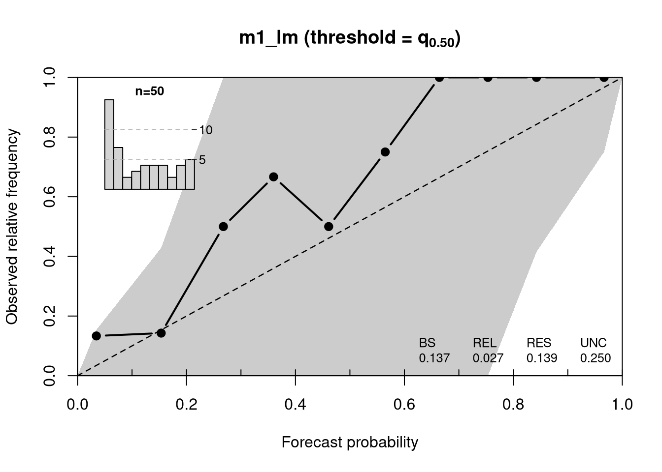
Reliagrams evaluate if a probability model is calibrated (reliable) by first partitioning the predicted probability for a binary event into a certain number of bins and then plotting (within each bin) the averaged forecast probability against the observered/empirical relative frequency. For computation, reliagram leverages the procast generic to forecast the respective predictive probabilities.

For continous probability forecasts, reliability diagrams can be computed either for a pre-specified threshold or for a specific quantile probability of the response values. Per default, reliagrams are computed for the 50%-quantile of the reponse.

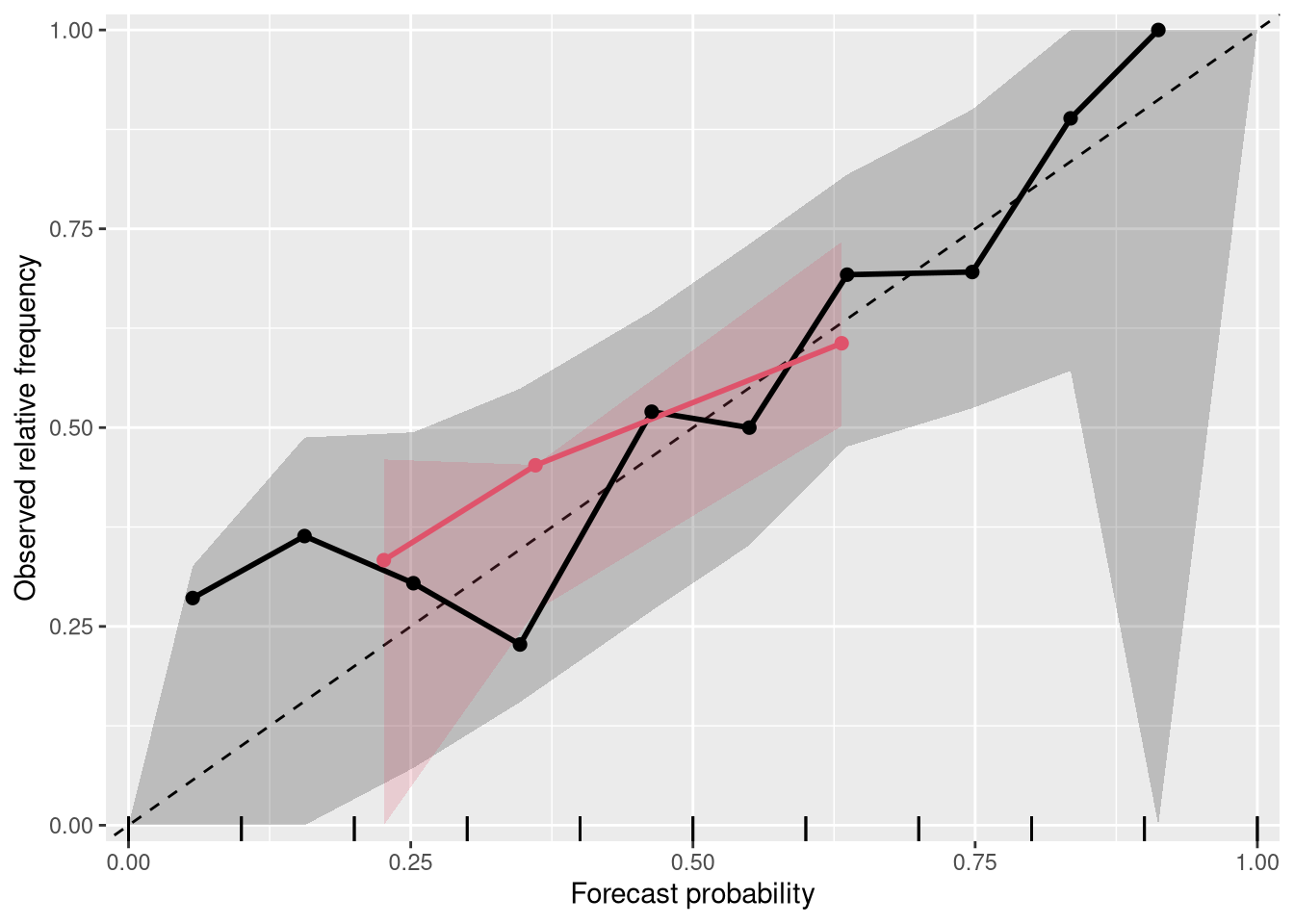
In addition to the plot and autoplot method for reliagram objects, it is also possible to combine two (or more) reliability diagrams by c/rbind, which creates a set of reliability diagrams that can then be plotted in one go.

Value

An object of class “reliagram” inheriting from “data.frame” or “tibble” conditional on the argument class with the following variables:

`x`	forecast probabilities,
`y`	observered/empirical relative frequencies,
`bin_lwr`, `bin_upr`	lower and upper bound of the binned forecast probabilities,
`n_pred`	number of predictions within the binned forecasts probabilites,
`ci_lwr`, `ci_upr`	lower and upper confidence interval bound.

Additionally, xlab, ylab, main, and treshold, confint_level, as well as the total and the decomposed Brier Score (bs, rel, res, unc) are stored as attributes.

Note

Note that there is also a reliability.plot function in the verification package. However, it only works for numeric forecast probabilities and numeric observed relative frequencies, hence a function has been created here.

References

Wilks DS (2011) Statistical Methods in the Atmospheric Sciences, 3rd ed., Academic Press, 704 pp.

Examples

library("topmodels")


## speed and stopping distances of cars
m1_lm <- lm(dist ~ speed, data = cars)

## compute and plot reliagram
reliagram(m1_lm)

#-------------------------------------------------------------------------------
## determinants for male satellites to nesting horseshoe crabs
data("CrabSatellites", package = "countreg")

## linear poisson model
m1_pois <- glm(satellites ~ width + color, data = CrabSatellites, family = poisson)
m2_pois <- glm(satellites ~ color, data = CrabSatellites, family = poisson)

## compute and plot reliagram as base graphic
r1 <- reliagram(m1_pois, plot = FALSE)
r2 <- reliagram(m2_pois, plot = FALSE)

## plot combined reliagram as "ggplot2" graphic
ggplot2::autoplot(c(r1, r2), single_graph = TRUE, col = c(1, 2), fill = c(1, 2))