S3 Methods for Plotting Rootograms

Description

Generic plotting functions for rootograms of the class “rootogram” computed by link{rootogram}.

Usage

## S3 method for class 'rootogram'
plot(
  x,
  style = NULL,
  scale = NULL,
  expected = NULL,
  ref = NULL,
  confint = NULL,
  confint_level = 0.95,
  confint_type = c("tukey", "pointwise", "simultaneous"),
  confint_nrep = 1000,
  xlim = c(NA, NA),
  ylim = c(NA, NA),
  xlab = NULL,
  ylab = NULL,
  main = NULL,
  axes = TRUE,
  box = FALSE,
  col = "darkgray",
  border = "black",
  lwd = 1,
  lty = 1,
  alpha_min = 0.8,
  expected_col = 2,
  expected_pch = 19,
  expected_lty = 1,
  expected_lwd = 2,
  confint_col = "black",
  confint_lty = 2,
  confint_lwd = 1.75,
  ref_col = "black",
  ref_lty = 1,
  ref_lwd = 1.25,
  ...
)

## S3 method for class 'rootogram'
autoplot(
  object,
  style = NULL,
  scale = NULL,
  expected = NULL,
  ref = NULL,
  confint = NULL,
  confint_level = 0.95,
  confint_type = c("tukey", "pointwise", "simultaneous"),
  confint_nrep = 1000,
  xlim = c(NA, NA),
  ylim = c(NA, NA),
  xlab = NULL,
  ylab = NULL,
  main = NULL,
  legend = FALSE,
  theme = NULL,
  colour = "black",
  fill = "darkgray",
  size = 0.5,
  linetype = 1,
  alpha = NA,
  expected_colour = 2,
  expected_size = 1,
  expected_linetype = 1,
  expected_alpha = 1,
  expected_fill = NA,
  expected_stroke = 0.5,
  expected_shape = 19,
  confint_colour = "black",
  confint_size = 0.5,
  confint_linetype = 2,
  confint_alpha = NA,
  ref_colour = "black",
  ref_size = 0.5,
  ref_linetype = 1,
  ref_alpha = NA,
  ...
)

Arguments

x, object	an object of class rootogram.
style	character specifying the syle of rootogram.
scale	character specifying whether raw frequencies or their square roots (default) should be drawn.
expected	Should the expected (fitted) frequencies be plotted?
ref	logical. Should a reference line be plotted?
confint	logical. Should confident intervals be drawn?
confint_level	numeric. The confidence level required.
confint_type	character. Should “tukey”, “pointwise”, or “simultaneous” confidence intervals be visualized?
confint_nrep	numeric. The repetition number of simulation for computing the confidence intervals.
xlim, ylim, xlab, ylab, main, axes, box	graphical parameters.
col, border, lwd, lty, alpha_min	graphical parameters for the histogram style part of the base plot.
expected_col, expected_pch, expected_lty, expected_lwd, ref_col, ref_lty, ref_lwd, expected_colour, expected_size, expected_linetype, expected_alpha, expected_fill, expected_stroke, expected_shape, ref_colour, ref_size, ref_linetype, ref_alpha, confint_col, confint_lty, confint_lwd, confint_colour, confint_size, confint_linetype, confint_alpha	Further graphical parameters for the ‘expected’ and ‘ref’ line using either autoplot or plot.
…	further graphical parameters passed to the plotting function.
legend	logical. Should a legend be added in the ggplot2 style graphic?
theme	Which ‘ggplot2’ theme should be used. If not set, theme_bw is employed.
colour, fill, size, linetype, alpha	graphical parameters for the histogram style part in the autoplot.

Details

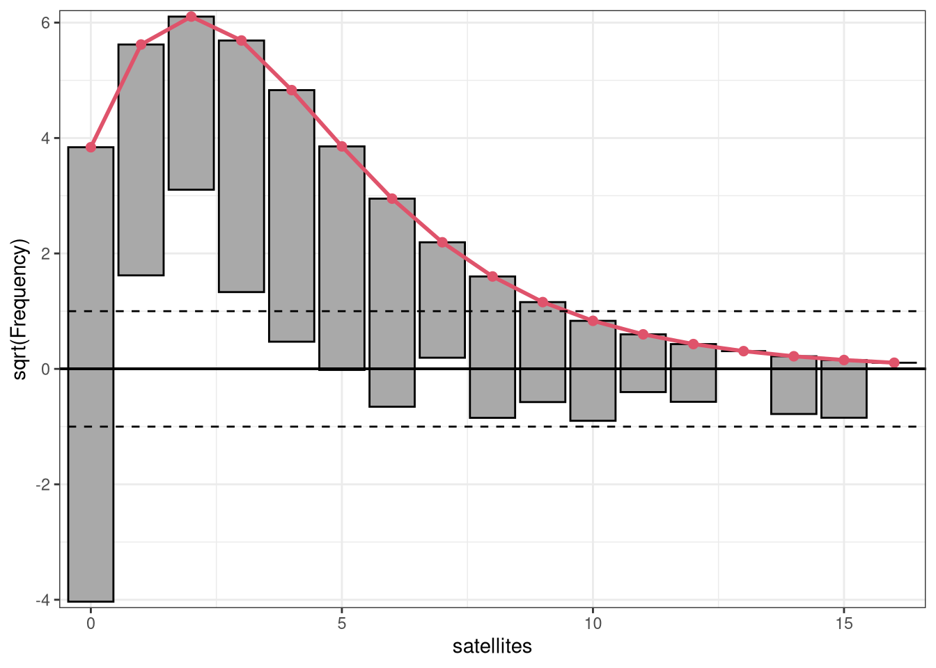
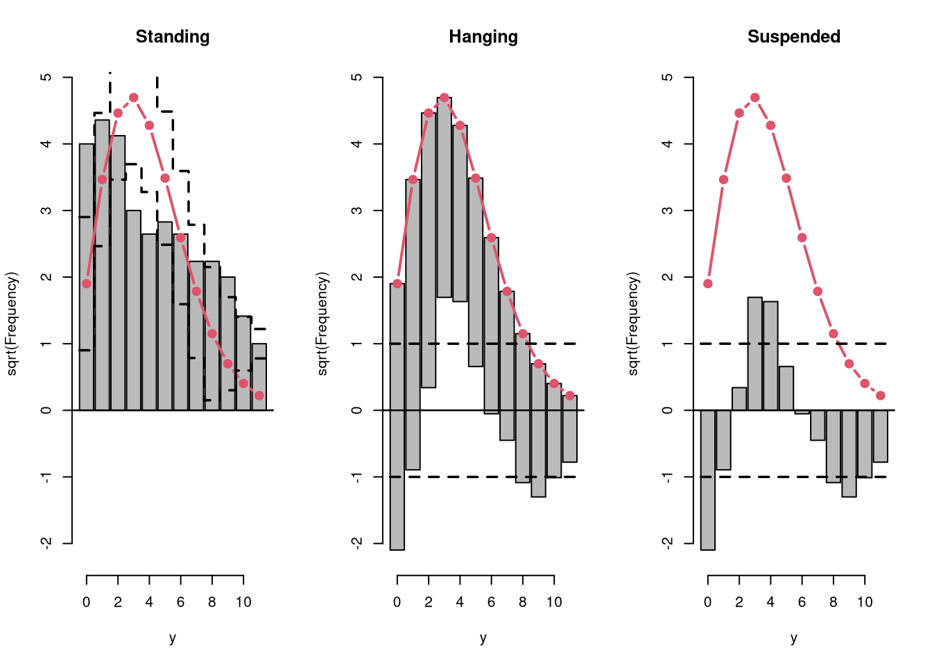
Rootograms graphically compare (square roots) of empirical frequencies with expected (fitted) frequencies from a probability model. For the observed distribution the histogram is drawn on a square root scale (hence the name) and superimposed with a line for the expected frequencies. The histogram can be “standing” on the x-axis (as usual), or “hanging” from the expected (fitted) curve, or a “suspended” histogram of deviations can be drawn.

Rootograms are associated with the work of John W. Tukey (see Tukey 1977) and were originally proposed for assessing the goodness of fit of univariate distributions and extended by Kleiber and Zeileis (2016) to regression setups.

As the expected distribution is typically a sum of different conditional distributions in regression models, the “pointwise” confidence intervals for each bin can be computed from mid-quantiles of a Poisson-Binomial distribution (Wilson and Einbeck 2021). Corresponding “simultaneous” confidence intervals for all bins can be obtained via simulation from the Poisson-Binomial distributions. As the pointwise confidence intervals are typically not substantially different from the warning limits of Tukey (1972, p. 61), set at +/- 1, these “tukey” intervals are used by default.

Note that for computing the exact “pointwise” intervals from the Poisson-Binomial distribution, the PoissonBinomial needs to be installed. Otherwise, a warning is issueed and a normal approximation is used.

References

Kleiber C, Zeileis A (2016). “Visualizing Count Data Regressions Using Rootograms.” The American Statistician, 70(3), 296–303. doi:10.1080/00031305.2016.1173590

Tukey JW (1972), “Some Graphic and Semigraphic Displays,” in Statistical Papers in Honor of George W. Snedecor, pp.293–316. Bancroft TA (Ed.). Iowa State University Press, Ames. Reprinted in William S. Cleveland (Ed.) (1988). The Collected Works of John W. Tukey, Volume V. Graphics: 1965–1985, Wadsworth & Brooks/Cole, Pacific Grove.

Tukey JW (1977). Exploratory Data Analysis. Addison-Wesley, Reading.

Wilson P, Einbeck J (2021). “A Graphical Tool for Assessing the Suitability of a Count Regression Model”, Austrian Journal of Statistics, 50(1), 1–23. doi:10.17713/ajs.v50i1.921

See Also

rootogram, procast

Examples

library("topmodels")


## speed and stopping distances of cars
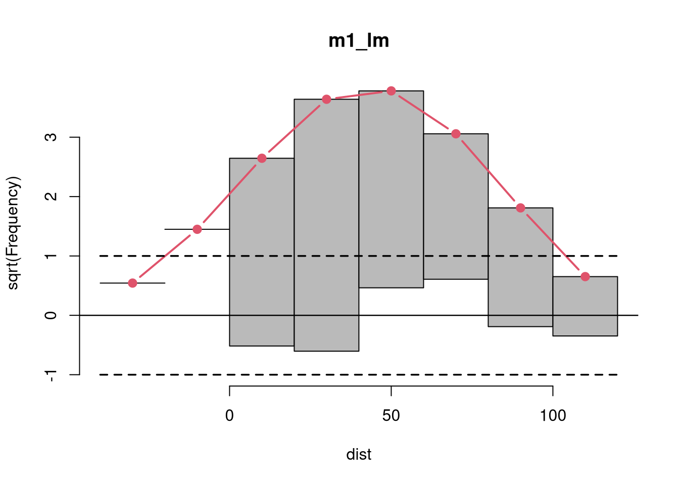
m1_lm <- lm(dist ~ speed, data = cars)

## compute and plot rootogram
rootogram(m1_lm)

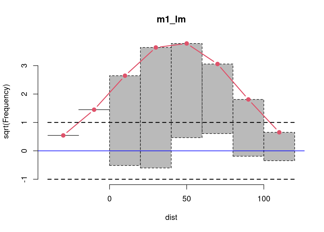
## customize colors
rootogram(m1_lm, ref_col = "blue", lty = 2, pch = 20)

#-------------------------------------------------------------------------------
if (require("crch")) {

  ## precipitation observations and forecasts for Innsbruck
  data("RainIbk", package = "crch")
  RainIbk <- sqrt(RainIbk)
  RainIbk$ensmean <- apply(RainIbk[, grep("^rainfc", names(RainIbk))], 1, mean)
  RainIbk$enssd <- apply(RainIbk[, grep("^rainfc", names(RainIbk))], 1, sd)
  RainIbk <- subset(RainIbk, enssd > 0)

  ## linear model w/ constant variance estimation
  m2_lm <- lm(rain ~ ensmean, data = RainIbk)

  ## logistic censored model
  m2_crch <- crch(rain ~ ensmean | log(enssd), data = RainIbk, left = 0, dist = "logistic")

  ### compute rootograms FIXME
  #r2_lm <- rootogram(m2_lm, plot = FALSE)
  #r2_crch <- rootogram(m2_crch, plot = FALSE)

  ### plot in single graph
  #plot(c(r2_lm, r2_crch), col = c(1, 2))
}

#-------------------------------------------------------------------------------
## determinants for male satellites to nesting horseshoe crabs
data("CrabSatellites", package = "countreg")

## linear poisson model
m3_pois <- glm(satellites ~ width + color, data = CrabSatellites, family = poisson)

## compute and plot rootogram as "ggplot2" graphic
rootogram(m3_pois, plot = "ggplot2")

#-------------------------------------------------------------------------------
## artificial data from negative binomial (mu = 3, theta = 2)
## and Poisson (mu = 3) distribution
set.seed(1090)
y <- rnbinom(100, mu = 3, size = 2)
x <- rpois(100, lambda = 3)

## glm method: fitted values via glm()
m4_pois <- glm(y ~ x, family = poisson)

## correctly specified Poisson model fit
par(mfrow = c(1, 3))
r4a_pois <- rootogram(m4_pois, style = "standing", ylim = c(-2.2, 4.8), main = "Standing")
r4b_pois <- rootogram(m4_pois, style = "hanging", ylim = c(-2.2, 4.8), main = "Hanging")
r4c_pois <- rootogram(m4_pois, style = "suspended", ylim = c(-2.2, 4.8), main = "Suspended")

par(mfrow = c(1, 1))