Methods for zerotrunc Objects

Description

Methods for extracting information from fitted zero-truncated count regression model objects of class “zerotrunc”.

Usage

## S3 method for class 'zerotrunc'
predict(object, newdata,
  type = c("response", "prob", "count", "zero"), na.action = na.pass, ...)
## S3 method for class 'zerotrunc'
residuals(object, type = c("deviance", "pearson", "response"), ...)

Arguments

object an object of class “zerotrunc” as returned by zerotrunc.
newdata optionally, a data frame in which to look for variables with which to predict. If omitted, the original observations are used.
type character specifying the type of predictions or residuals, respectively. For details see below.
na.action function determining what should be done with missing values in newdata. The default is to predict NA.
currently not used.

Details

A set of standard extractor functions for fitted model objects is available for objects of class “zerotrunc”, including methods to the generic functions print and summary which print the estimated coefficients along with some further information. The summary in particular supplies partial Wald tests based on the coefficients and the covariance matrix (estimated from the Hessian in the numerical optimization of the log-likelihood). As usual, the summary method returns an object of class “summary.zerotrunc” containing the relevant summary statistics which can subsequently be printed using the associated print method.

Both the fitted and predict methods can compute fitted responses. The latter additionally provides the predicted density (i.e., probabilities for the observed counts), the predicted mean from the count component (without zero truncation) and the predicted probability for observing a non-zero count (in the un-truncated model). The residuals method can compute raw residuals (observed - fitted), Pearson residuals (raw residuals scaled by square root of variance function), and deviance residuals (contributions to the centered log-likelihood).

A logLik method is provided, hence AIC can be called to compute information criteria.
See Also

zerotrunc

Examples

library("countreg")

data("CrabSatellites", package = "countreg")
fm <- zerotrunc(satellites ~ width + color, data = CrabSatellites, subset = satellites > 0)

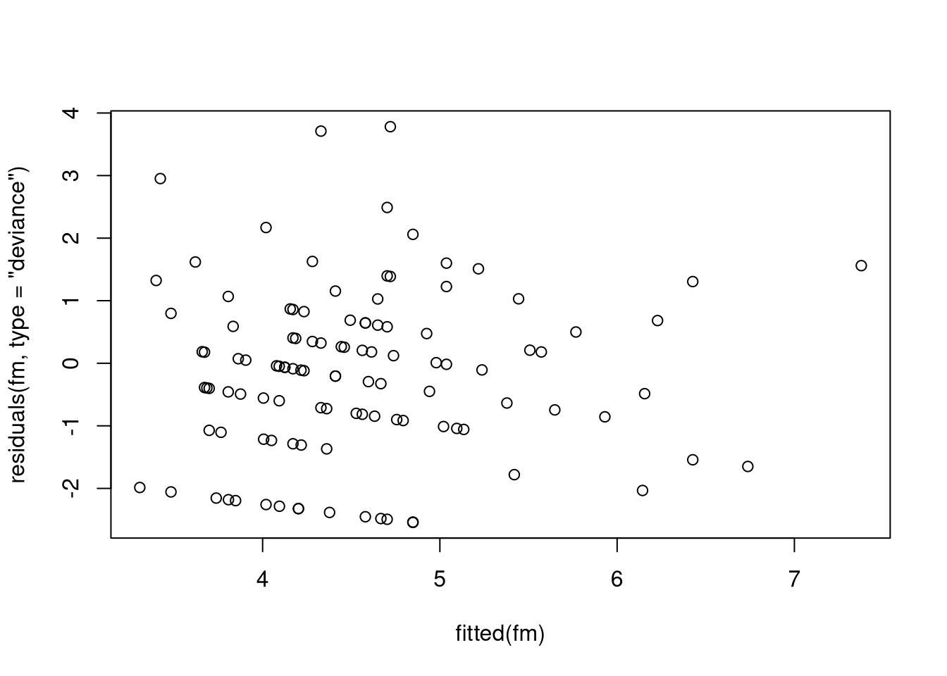
plot(residuals(fm, type = "deviance") ~ fitted(fm))

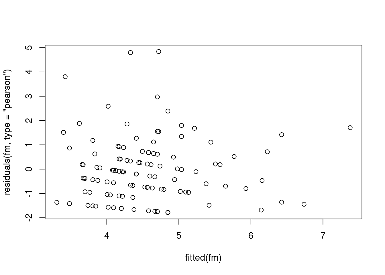
plot(residuals(fm, type = "pearson") ~ fitted(fm))

coef(fm)
(Intercept)       width     color.L     color.Q     color.C 
 0.52666751  0.03971107  0.10777950  0.39487848  0.16936889 

Call:
zerotrunc(formula = satellites ~ width + color, data = CrabSatellites, 
    subset = satellites > 0)

Deviance residuals:
    Min      1Q  Median      3Q     Max 
-2.5416 -1.0496 -0.1063  0.6271  3.7814 

Coefficients (truncated poisson with log link):
            Estimate Std. Error z value Pr(>|z|)   
(Intercept)  0.52667    0.60017   0.878  0.38020   
width        0.03971    0.02228   1.783  0.07466 . 
color.L      0.10778    0.14402   0.748  0.45425   
color.Q      0.39488    0.12110   3.261  0.00111 **
color.C      0.16937    0.09365   1.808  0.07054 . 
---
Signif. codes:  0 '***' 0.001 '**' 0.01 '*' 0.05 '.' 0.1 ' ' 1

Number of iterations in BFGS optimization: 8 
Log-likelihood: -261.9 on 5 Df
logLik(fm)
'log Lik.' -261.9177 (df=5)
AIC(fm)
[1] 533.8354