Extension of the Binomial Distribution

Description

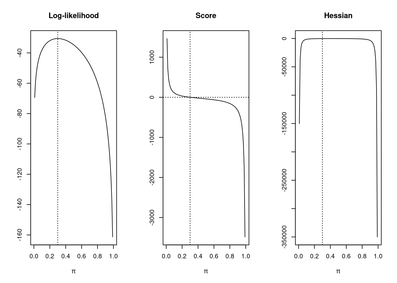
Score function, hessian, mean, and variance for the binomial distribution with parameters prob and size.

Usage

sbinom(x, prob, size, parameter = "prob", drop = TRUE)
hbinom(x, prob, size, parameter = "prob", drop = TRUE)
mean_binom(prob, size, drop = TRUE)
var_binom(prob, size, drop = TRUE)

Arguments

x	vector of quantiles.
prob	probability of success on each trial.
size	number of trials (zero or more).
parameter	character. Derivatives are computed wrt this paramter. Note: Only “prob” is implemented.
drop	logical. Should the result be a matrix (drop = FALSE) or should the dimension be dropped (drop = TRUE, the default)?

Details

The binomial distribution with size \(= n\) and prob \(= p\) has density

\(p(x) = {n \choose x} {p}^{x} {(1-p)}^{n-x}\)

for \(x = 0, \ldots, n\).

The score function is

\(s(p) = \frac{x}{p} - \frac{n-x}{1-p}\)

The hessian is

\(h(p) = - \frac{x}{p^2} - \frac{n-x}{(1-p)^2}\)

Value

sbinom gives the score function, i.e., the 1st derivative of the log-density wrt prob and hbinom gives the hessian, i.e., the 2nd derivative of the log-density wrt prob. mean and var give the mean and variance, respectively.

See Also

Binomial encompassing dbinom, pbinom, qbinom and rbinom.

Examples

library("countreg")

## Simulate some data
set.seed(123)
y <- rbinom(50, size = 1, prob = 0.3)

## Plot log-likelihood function
par(mfrow = c(1,3))
ll <- function(x) {sum(dbinom(y, size = 1, prob = x, log = TRUE))}
curve(sapply(x, ll), xlab = expression(pi), ylab = "", main = "Log-likelihood")
abline(v = 0.3, lty = 3)

## Plot score function
curve(sapply(x, function(x) sum(sbinom(y, size = 1, x))),
      xlab = expression(pi), ylab = "", main = "Score")
abline(h = 0, lty = 3)
abline(v = 0.3, lty = 3)

## Plot hessian
curve(sapply(x, function(x) sum(hbinom(y, size = 1, x))),
      xlab = expression(pi), ylab = "", main = "Hessian")
abline(v = 0.3, lty = 3)