Determinants for male satellites to nesting horseshoe crabs.
Usage
data("CrabSatellites")
Format
A data frame containing 173 observations on 5 variables.
color
Ordered factor indicating color (light medium, medium, dark medium, dark).
spine
Ordered factor indicating spine condition (both good, one worn or broken, both worn or broken).
width
Carapace width (cm).
weight
Weight (kg).
satellites
Number of satellites.
Details
Brockmann (1996) investigates horshoe crab mating. The crabs arrive on the beach in pairs to spawn. Furthermore, unattached males also come to the beach, crowd around the nesting couples and compete with attached males for fertilizations. These so-called satellite males form large groups around some couples while ignoring others. Brockmann (1996) shows that the groupings are not driven by environmental factors but by properties of the nesting female crabs. Larger females that are in better condition attract more satellites.
Agresti (2002, 2013) reanalyzes the number of satellites using count models. Explanatory variables are the female crab’s color, spine condition, weight, and carapace width. Color and spine condition are ordered factors but are treated as numeric in some analyses.
Source
Table 4.3 in Agresti (2002).
References
Agresti A (2002). Categorical Data Analysis, 2nd ed., John Wiley & Sons, Hoboken.
Agresti A (2013). Categorical Data Analysis, 3rd ed., John Wiley & Sons, Hoboken.
Brockmann HJ (1996). “Satellite Male Groups in Horseshoe Crabs, Limulus polyphemus”, Ethology, 102(1), 1–21.
Examples
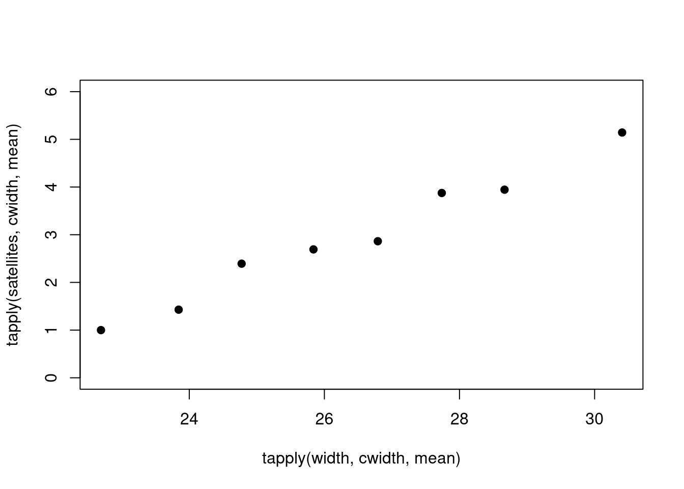
library("countreg")## load data, use ordered factors as numeric, and## grouped factor version of widthdata("CrabSatellites", package ="countreg")CrabSatellites<-transform(CrabSatellites, color =as.numeric(color), spine =as.numeric(spine), cwidth =cut(width, c(-Inf, seq(23.25, 29.25), Inf)))## Agresti, Table 4.4aggregate(CrabSatellites$satellites, list(CrabSatellites$cwidth), function(x)round(c(Number =length(x), Sum =sum(x), Mean =mean(x), Var =var(x)), digits =2))
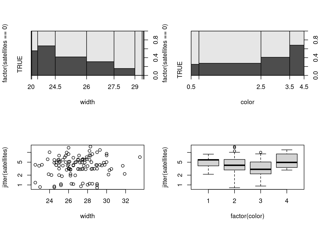
## alternatively: exploratory displays for hurdle (= 0 vs. > 0) and counts (> 0)par(mfrow =c(2, 2))plot(factor(satellites==0)~width, data =CrabSatellites, breaks =seq(20, 33.5, by =1.5))plot(factor(satellites==0)~color, data =CrabSatellites, breaks =1:5-0.5)plot(jitter(satellites)~width, data =CrabSatellites, subset =satellites>0, log ="y")plot(jitter(satellites)~factor(color), data =CrabSatellites, subset =satellites>0, log ="y")
## count data modelscs_p<-glm(satellites~width+color, data =CrabSatellites, family =poisson)cs_nb<-glm.nb(satellites~width+color, data =CrabSatellites)cs_hp<-hurdle(satellites~width+color, data =CrabSatellites, dist ="poisson")cs_hnb<-hurdle(satellites~width+color, data =CrabSatellites, dist ="negbin")cs_hnb2<-hurdle(satellites~1|width+color, data =CrabSatellites, dist ="negbin")AIC(cs_p, cs_nb, cs_hp, cs_hnb, cs_hnb2)
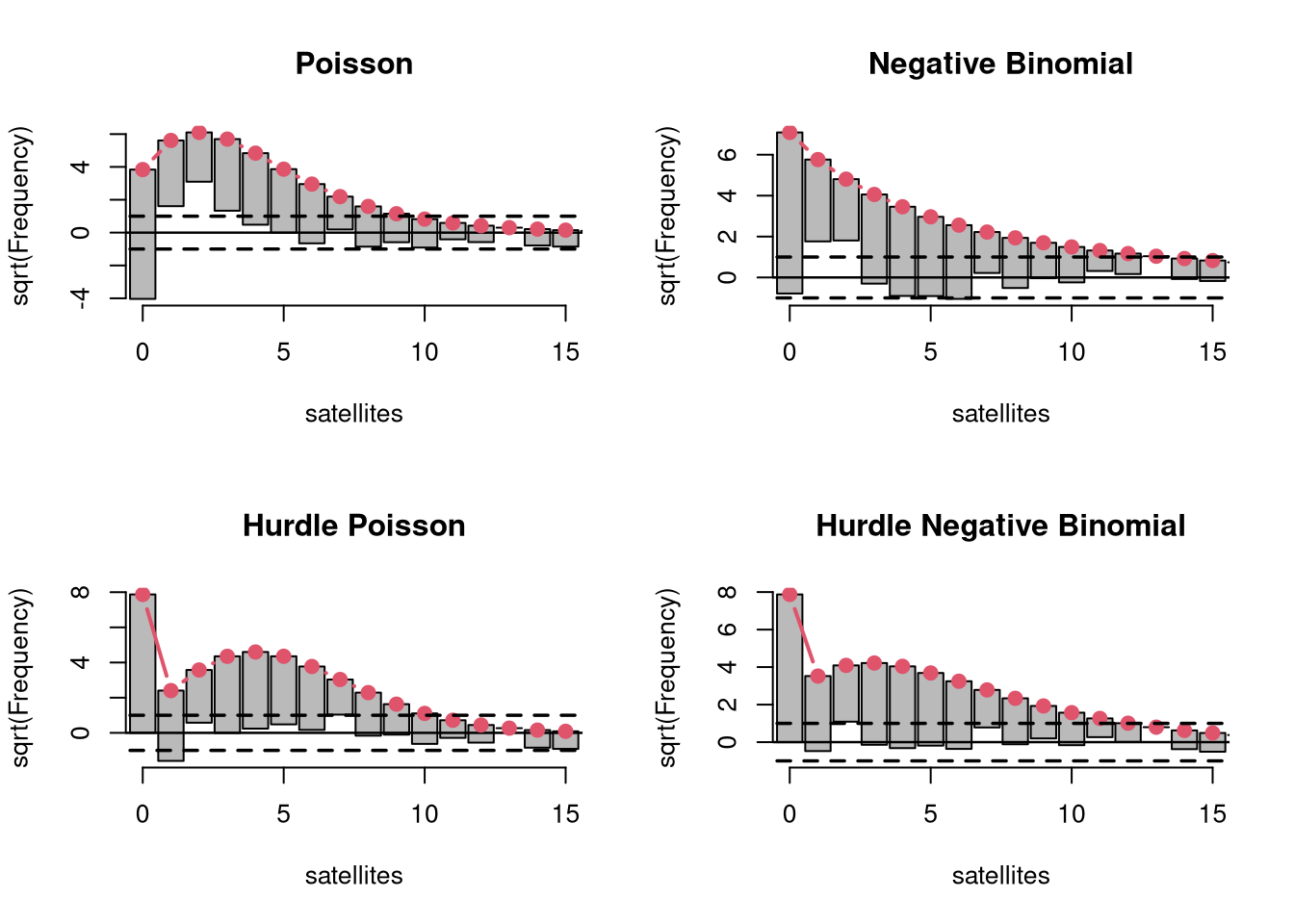
## rootogramsif(require("topmodels")){par(mfrow =c(2, 2))r_p<-rootogram(cs_p, xlim =c(0, 15), main ="Poisson")r_nb<-rootogram(cs_nb, xlim =c(0, 15), main ="Negative Binomial")r_hp<-rootogram(cs_hp, xlim =c(0, 15), main ="Hurdle Poisson")r_hnb<-rootogram(cs_hnb, xlim =c(0, 15), main ="Hurdle Negative Binomial")}
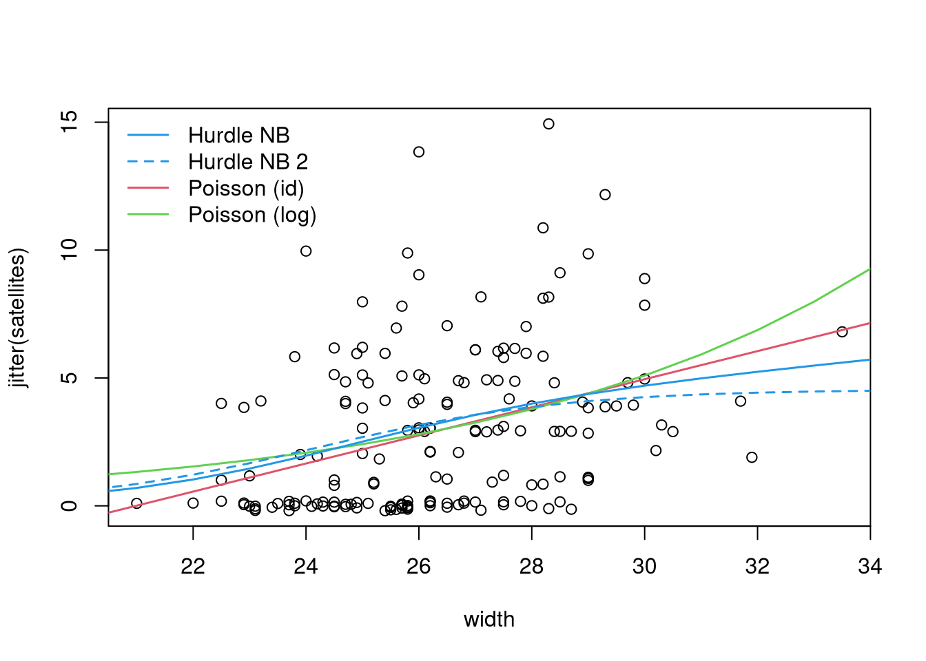
## fitted curvespar(mfrow =c(1, 1))plot(jitter(satellites)~width, data =CrabSatellites)nd<-data.frame(width =20:34, color =2)pred<-function(m)predict(m, newdata =nd, type ="response")cs_ag<-glm(satellites~width, data =CrabSatellites, family =poisson(link ="identity"), start =coef(lm(satellites~width, data =CrabSatellites)))lines(pred(cs_ag)~width, data =nd, col =2, lwd =1.5)lines(pred(cs_p)~width, data =nd, col =3, lwd =1.5)lines(pred(cs_hnb)~width, data =nd, col =4, lwd =1.5)lines(pred(cs_hnb2)~width, data =nd, col =4, lwd =1.5, lty =2)legend("topleft", c("Hurdle NB", "Hurdle NB 2", "Poisson (id)", "Poisson (log)"), col =c(4, 4, 2, 3), lty =c(1, 2, 1, 1), lwd =1.5, bty ="n")
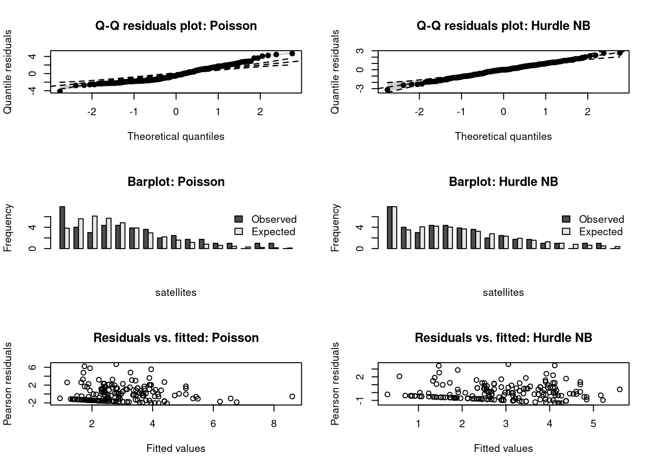
## alternative displays: Q-Q residuals plot, barplot, residuals vs. fittedif(require("topmodels")){par(mfrow=c(3, 2))qqrplot(cs_p, range =c(0.05, 0.95), main ="Q-Q residuals plot: Poisson")qqrplot(cs_hnb, range =c(0.05, 0.95), main ="Q-Q residuals plot: Hurdle NB")}else{par(mfrow=c(2, 2))}barplot(t(matrix(c(r_p$observed, r_p$expected), ncol =2, dimnames =list(r_p$x, c("Observed", "Expected")))), beside =TRUE, main ="Barplot: Poisson", xlab ="satellites", ylab ="Frequency", legend.text =TRUE, args.legend =list(x ="topright", bty ="n"))barplot(t(matrix(c(r_hnb$observed, r_hnb$expected), ncol =2, dimnames =list(r_hnb$x, c("Observed", "Expected")))), beside =TRUE, main ="Barplot: Hurdle NB", xlab ="satellites", ylab ="Frequency", legend.text =TRUE, args.legend =list(x ="topright", bty ="n"))plot(predict(cs_p, type ="response"),residuals(cs_p, type ="pearson"), xlab ="Fitted values", ylab ="Pearson residuals", main ="Residuals vs. fitted: Poisson")plot(predict(cs_hnb, type ="response"),residuals(cs_hnb, type ="pearson"), xlab ="Fitted values", ylab ="Pearson residuals", main ="Residuals vs. fitted: Hurdle NB")