Extension of the Negative Binomial Distribution

Description

Score function, hessian, mean, and variance for the negative binomial distribution with parameters mu and size.

Usage

snbinom(x, mu, size, parameter = c("mu", "size"), drop = TRUE)
hnbinom(x, mu, size, parameter = c("mu", "size"), drop = TRUE)
mean_nbinom(mu, size, drop = TRUE)
var_nbinom(mu, size, drop = TRUE)

Arguments

x	vector of quantiles.
mu	mean of distribution.
size	dispersion parameter. Must be strictly positive.
parameter	character. Derivatives are computed wrt this paramter.
drop	logical. Should the result be a matrix (drop = FALSE) or should the dimension be dropped (drop = TRUE, the default)?

Details

The negative binomial with mu and size (or theta) has density

f(y | , ) = , y {0, 1, 2, }

Derivatives of the log-likelihood \(\ell\) wrt \(\mu\):

= -

= - +

Derivatives wrt \(\theta\):

= _0(y + ) - _0() + () + 1 - (+ ) -

= _1(y + ) - _1() + - +

\(\psi_0\) and \(\psi_1\) denote the digamma and trigamma function, respectively.

The derivative wrt \(\mu\) and \(\theta\):

= =

Value

snbinom gives the score function, i.e., the 1st derivative of the log-density wrt mu or theta and hnbinom gives the hessian, i.e., the 2nd derivative of the log-density wrt mu and/or theta. mean and var give the mean and variance, respectively.

Note

No parameter prob—as in dnbinom, pnbinom, qnbinom and rnbinom—is implemented in the functions snbinom and hnbinom.

See Also

NegBinomial encompassing dnbinom, pnbinom, qnbinom and rnbinom.

Examples

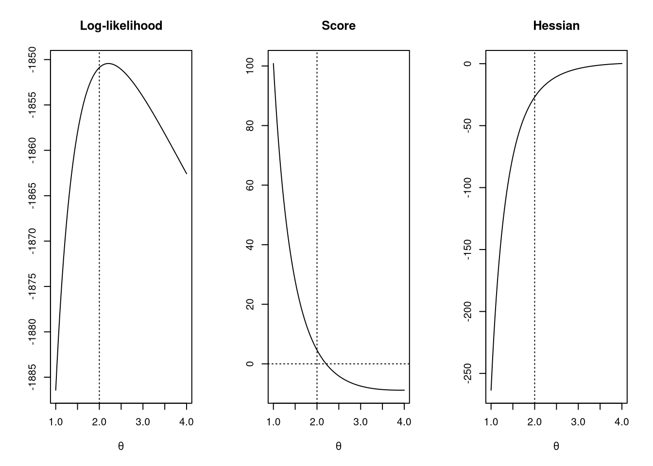
library("countreg")

## Simulate some data
set.seed(123)
y <- rnbinom(1000, size = 2, mu = 2)

## Plot log-likelihood function
par(mfrow = c(1, 3))
ll <- function(x) {sum(dnbinom(y, size = x, mu = 2, log = TRUE))}
curve(sapply(x, ll), 1, 4, xlab = expression(theta), ylab = "",
      main = "Log-likelihood")
abline(v = 2, lty = 3)

## Plot score function
curve(sapply(x, function(x) sum(snbinom(y, size = x, mu = 2, parameter = "size"))),
      1, 4, xlab = expression(theta), ylab = "", main = "Score")
abline(h = 0, lty = 3)
abline(v = 2, lty = 3)

## Plot hessian
curve(sapply(x, function(x) sum(hnbinom(y, size = x, mu = 2, parameter = "size"))),
      1, 4, xlab = expression(theta), ylab = "", main = "Hessian")
abline(v = 2, lty = 3)