Basics

\[ \newcommand{\E}{\mathsf{E}} \newcommand{\VAR}{\mathsf{VAR}} \newcommand{\COV}{\mathsf{COV}} \newcommand{\Prob}{\mathsf{P}} \]

1 Generalized linear models

The basic count data regression models can be represented and understood using the GLM framework that emerged in the statistical literature in the early 1970s (Nelder and Wedderburn 1972). In the following, we briefly sketch some important aspects relating to the unifying conceptual properties and their implementation in R—for a detailed theoretical account of GLMs see McCullagh and Nelder (1989).

GLMs describe the dependence of a scalar variable \(y_i\) (\(i = 1, \dots, n\)) on a vector of regressors \(x_i\). The conditional distribution of \(y_i | x_i\) is a linear exponential family with probability density function \[ f(y; \lambda, \phi) \quad = \quad \exp \left( \frac{y \cdot \lambda - b(\lambda)}{\phi} + c(y, \phi) \right), \tag{1}\] where \(\lambda\) is the canonical parameter that depends on the regressors via a linear predictor and \(\phi\) is a dispersion parameter that is often known. The functions \(b(\cdot)\) and \(c(\cdot)\) are known and determine which member of the family is used, e.g., the normal, binomial or Poisson distribution. Conditional mean and variance of \(y_i\) are given by \(\E[y_i \, | \, x_i] = \mu_i = b'(\lambda_i)\) and \(\VAR[y_i \, | \, x_i] = \phi \cdot b''(\lambda_i)\). Thus, up to a scale or dispersion parameter \(\phi\), the distribution of \(y_i\) is determined by its mean. Its variance is proportional to \(V(\mu) = b''(\lambda(\mu))\), also called variance function.

The dependence of the conditional mean \(\E[y_i \, | \, x_i] = \mu_i\) on the regressors \(x_i\) is specified via \[ g(\mu_i) \quad = \quad x_i^\top \beta, \tag{2}\] where \(g(\cdot)\) is a known link function and \(\beta\) is the vector of regression coefficients which are typically estimated by maximum likelihood (ML) using the iterative weighted least squares (IWLS) algorithm.

Instead of viewing GLMs as models for the full likelihood (as determined by Equation 1), they can also be regarded as regression models for the mean only (as specified in Equation 2) where the estimating functions used for fitting the model are derived from a particular family. As illustrated in the remainder of this section, the estimating function point of view is particularly useful for relaxing the assumptions imposed by the Poisson likelihood.

R provides a very flexible implementation of the general GLM framework in the function glm() (Chambers and Hastie 1992) contained in the stats package. Its most important arguments are

where formula plus data is the now standard way of specifying regression relationships in R/S introduced in Chambers and Hastie (1992). The remaining arguments in the first line (subset, na.action, weights, and offset) are also standard for setting up formula-based regression models in R/S. The arguments in the second line control aspects specific to GLMs while the arguments in the last line specify which components are returned in the fitted model object (of class glm which inherits from lm). By default the model frame (model) and the vector \((y_1, \dots, y_n)^\top\) (y) but not the model matrix (x, containing \(x_1, \dots, x_n\) combined row-wise) are included. The family argument specifies the link \(g(\mu)\) and variance function \(V(\mu)\) of the model, start can be used to set starting values for \(\beta\), and control contains control parameters for the IWLS algorithm. For further arguments to glm() (including alternative specifications of starting values) see ?glm. The high-level glm() interface relies on the function glm.fit() which carries out the actual model fitting (without taking a formula-based input or returning classed output).

For glm objects, a set of standard methods (including print(), predict(), logLik() and many others) are provided. Inference can easily be performed using the summary() method for assessing the regression coefficients via partial Wald tests or the anova() method for comparing nested models via an analysis of deviance. These inference functions are complemented by further generic inference functions in contributed packages: e.g., lmtest (Zeileis and Hothorn 2002) provides a coeftest() function that also computes partial Wald tests but allows for specification of alternative (robust) standard errors. Similarly, waldtest() from lmtest and linearHypothesis() from car (Fox 2002) assess nested models via Wald tests (using different specifications for the nested models). Finally, lrtest() from lmtest compares nested models via likelihood ratio (LR) tests based on an interface similar to waldtest() and anova().

2 Poisson Model

The simplest distribution used for modeling count data is the Poisson distribution with probability density function \[ f(y; \mu) \quad = \quad \frac{\exp(-\mu) \cdot \mu^{y}}{y!}, \tag{3}\] which is of type (1) and thus Poisson regression is a special case of the GLM framework. The canonical link is \(g(\mu) = \log(\mu)\) resulting in a log-linear relationship between mean and linear predictor. The variance in the Poisson model is identical to the mean, thus the dispersion is fixed at \(\phi = 1\) and the variance function is \(V(\mu) = \mu\).

In R, this can easily be specified in the glm() call just by setting family = poisson (where the default log link could also be changed in the poisson() call).

In practice, the Poisson model is often useful for describing the mean \(\mu_i\) but underestimates the variance in the data, rendering all model-based tests liberal. One way of dealing with this is to use the same estimating functions for the mean, but to base inference on the more robust sandwich covariance matrix estimator. In R, this estimator is provided by the sandwich() function in the sandwich package (Zeileis 2004, 2006).

3 Quasi-Poisson model

Another way of dealing with over-dispersion is to use the mean regression function and the variance function from the Poisson GLM but to leave the dispersion parameter \(\phi\) unrestricted. Thus, \(\phi\) is not assumed to be fixed at \(1\) but is estimated from the data. This strategy leads to the same coefficient estimates as the standard Poisson model but inference is adjusted for over-dispersion. Consequently, both models (quasi-Poisson and sandwich-adjusted Poisson) adopt the estimating function view of the Poisson model and do not correspond to models with fully specified likelihoods.

In R, the quasi-Poisson model with estimated dispersion parameter can also be fitted with the glm() function, simply setting family = quasipoisson.

4 Negative binomial models

A third way of modeling over-dispersed count data is to assume a negative binomial (NB) distribution for \(y_i | x_i\) which can arise as a gamma mixture of Poisson distributions. One parameterization of its probability density function is \[ f(y; \mu, \theta) \quad = \quad \frac{\Gamma(y + \theta)}{\Gamma(\theta) \cdot y!} \cdot \frac{\mu^{y} \cdot \theta^\theta}{(\mu + \theta)^{y + \theta}}, \tag{4}\] with mean \(\mu\) and shape parameter \(\theta\); \(\Gamma(\cdot)\) is the gamma function. For every fixed \(\theta\), this is of type (1) and thus is another special case of the GLM framework. It also has \(\phi = 1\) but with variance function \(V(\mu) = \mu + \frac{\mu^2}{\theta}\).

Package MASS (Venables and Ripley 2002) provides the family function negative.binomial() that can directly be plugged into glm() provided the argument theta is specified. One application would be the geometric model, the special case where \(\theta = 1\), which can consequently be fitted in R by setting family = negative.binomial(theta = 1) in the glm() call.

If \(\theta\) is not known but to be estimated from the data, the negative binomial model is not a special case of the general GLM—however, an ML fit can easily be computed re-using GLM methodology by iterating estimation of \(\beta\) given \(\theta\) and vice versa. This leads to ML estimates for both \(\beta\) and \(\theta\) which can be computed using the function glm.nb() from the package MASS. It returns a model of class negbin inheriting from glm for which appropriate methods to the generic functions described above are again available.

5 Illustrations

In the following, we illustrate all models described above by applying them to a cross-sectional data set from health economics. Before the parametric models are fitted, a basic exploratory analysis of the data set is carried out that addresses some problems typically encountered when visualizing count data. At the end of the section, all fitted models are compared highlighting that the modelled mean function is similar but the fitted likelihood is different and thus, the models differ with respect to explaining over-dispersion.

Deb and Trivedi (1997) analyze data on 4406 individuals, aged 66 and over, who are covered by Medicare, a public insurance program. Originally obtained from the US National Medical Expenditure Survey (NMES) for 1987/88, the data are available from the data archive of the Journal of Applied Econometrics at https://journaldata.zbw.eu/dataset/demand-for-medical-care-by-the-elderly-a-finite-mixture-approach. It was prepared for the R package AER accompanying Kleiber and Zeileis (2008) and is also available as DebTrivedi.rda in the Journal of Statistical Software together with Zeileis (2006). The objective is to model the demand for medical care—as captured by the number of physician/non-physician office and hospital outpatient visits—by the covariates available for the patients. Here, we adopt the number of physician office visits visits as the dependent variable and use the health status variables¹ health (self-perceived health status), chronic (number of chronic conditions), as well as the socio-economic variables gender, school (number of years of education), and insurance (private insurance indicator) as regressors. For convenience, we select the variables used from the full data set:

data("NMES1988", package = "AER")
dt <- NMES1988[, c(1, 7, 8, 13, 15, 18)]

To obtain a first overview of the dependent variable, we employ a histogram of the observed count frequencies. In R various tools could be used, e.g., hist(dt$visits, breaks = 0:90 - 0.5) for a histogram with rectangles or

plot(table(dt$visits))

(see Figure 1) for a histogram with lines which brings out the extremely large counts somewhat better. The histogram illustrates that the marginal distribution exhibits both substantial variation and a rather large number of zeros.

Figure 1: Frequency distribution for number of physician office visits.

Figure 2: Bivariate explorative displays for number of physician office visits plotted against number of chronic conditions.

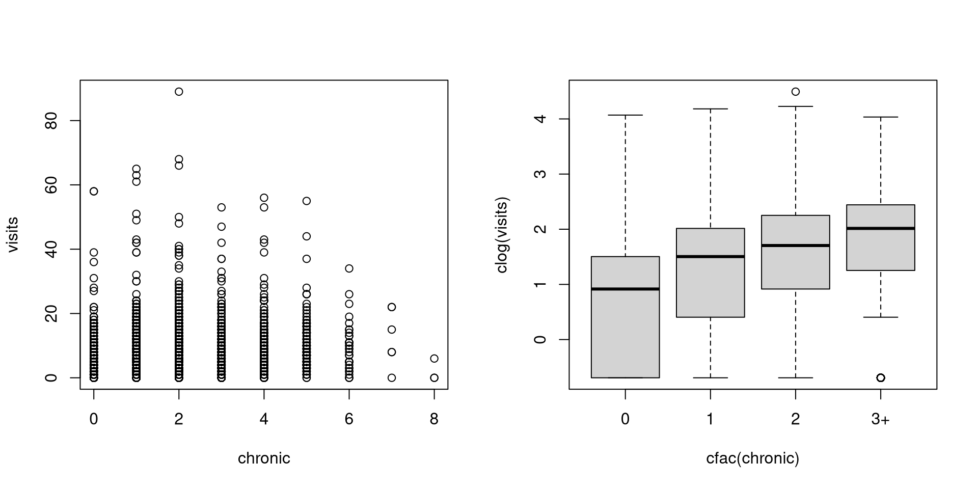
A natural second step in the exploratory analysis is to look at pairwise bivariate displays of the dependent variable against each of the regressors bringing out the partial relationships. In R, such bivariate displays can easily be generated with the plot() method for formulas, e.g., via plot(y ~ x). This chooses different types of displays depending on the combination of quantitative and qualitative variables as dependent or regressor variable, respectively. However, count variables are treated as all numerical variables and therefore the command

plot(visits ~ chronic, data = dt)

produces a simple scatterplot as shown in the left panel of Figure 2. This is clearly not useful as both variables are count variables producing numerous ties in the bivariate distribution and thus obscuring a large number of points in the display. To overcome the problem, it is useful to group the number of chronic conditions into a factor with levels 0',1’, 2', and3 or more’ and produce a boxplot instead of a scatterplot. Furthermore, the picture is much clearer if the dependent variable is log-transformed (just as all count regression models discussed above also use a log link by default). As there are zero counts as well, we use a convenience function clog() providing a continuity-corrected logarithm.

clog <- function(x) log(x + 0.5)

For transforming a count variable to a factor (for visualization purposes only), we define another convenience function cfac()

cfac <- function(x, breaks = NULL) {
  if(is.null(breaks)) breaks <- unique(quantile(x, 0:10/10))
  x <- cut(x, breaks, include.lowest = TRUE, right = FALSE)
  levels(x) <- paste(breaks[-length(breaks)], ifelse(diff(breaks) > 1,
    c(paste("-", breaks[-c(1, length(breaks))] - 1, sep = ""), "+"), ""),
    sep = "")
  return(x)
}

which by default tries to take an educated guess how to choose the breaks between the categories. Clearly, the resulting exploratory display of the transformed variables produced by

plot(clog(visits) ~ cfac(chronic), data = dt)

(shown in the right panel of Figure 2) brings out much better how the number of doctor visits increases with the number of chronic conditions.

Figure 3: Number of physician office visits plotted against regressors used.

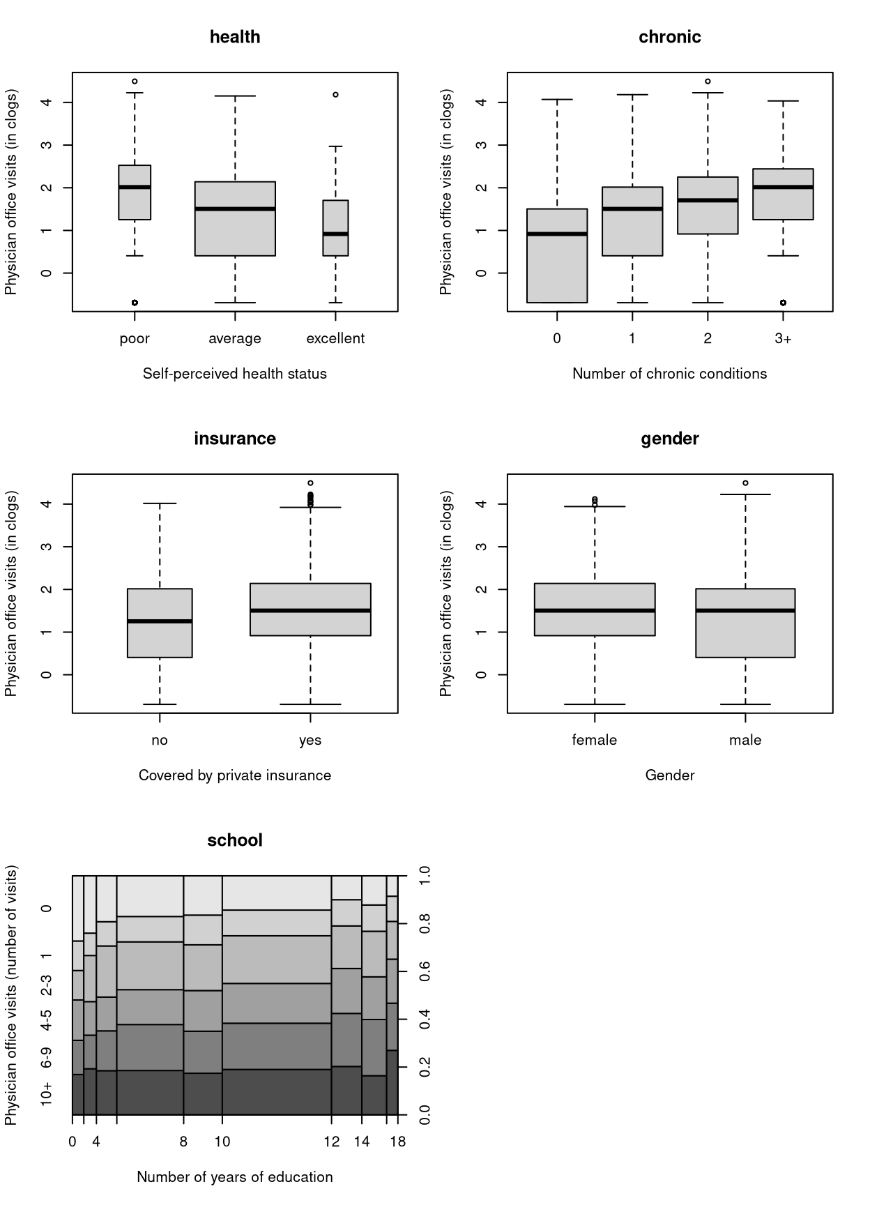
Analogous displays for the number of physician office visits against all regressors can be produced via

plot(clog(visits) ~ health, data = dt, varwidth = TRUE)
plot(clog(visits) ~ cfac(chronic), data = dt)
plot(clog(visits) ~ insurance, data = dt, varwidth = TRUE)
plot(clog(visits) ~ gender, data = dt, varwidth = TRUE)
plot(cfac(visits, c(0:2, 4, 6, 10, 100)) ~ school, data = dt, breaks = 9)

and are shown (with slightly enhanced labeling) in Figure 3. The last plot uses a different type of display. Here, the dependent count variable is not log-transformed but grouped into a factor and then a spinogram is produced. This also groups the regressor (as in a histogram) and then produces a highlighted mosaic plot. All displays show that the number of doctor visits increases or decreases with the regressors as expected: visits decreases with the general health status but increases with the number of chronic conditions or hospital stays. The median number of visits is also slightly higher for patients with a private insurance and higher level of education. It is slightly lower for male compared to female patients. The overall impression from all displays is that the changes in the mean can only explain a modest amount of variation in the data.

5.1 Poisson regression

As a first attempt to capture the relationship between the number of physician office visits and all regressors—described in R by the formula visits ~ .—in a parametric regression model, we fit the basic Poisson regression model

fm_pois <- glm(visits ~ ., data = dt, family = poisson)

and obtain the coefficient estimates along with associated partial Wald tests

summary(fm_pois)

Call:
glm(formula = visits ~ ., family = poisson, data = dt)

Coefficients:
                 Estimate Std. Error z value Pr(>|z|)    
(Intercept)      1.034542   0.023857  43.364   <2e-16 ***
healthpoor       0.318205   0.017479  18.205   <2e-16 ***
healthexcellent -0.379045   0.030291 -12.514   <2e-16 ***
chronic          0.168793   0.004471  37.755   <2e-16 ***
gendermale      -0.108014   0.012943  -8.346   <2e-16 ***
school           0.025754   0.001843  13.972   <2e-16 ***
insuranceyes     0.216007   0.016872  12.803   <2e-16 ***
---
Signif. codes:  0 '***' 0.001 '**' 0.01 '*' 0.05 '.' 0.1 ' ' 1

(Dispersion parameter for poisson family taken to be 1)

    Null deviance: 26943  on 4405  degrees of freedom
Residual deviance: 23808  on 4399  degrees of freedom
AIC: 36597

Number of Fisher Scoring iterations: 5

All coefficient estimates confirm the results from the exploratory analysis in Figure 3. All coefficients are highly significant with the health variables leading to somewhat larger Wald statistics compared to the socio-economic variables. However, the Wald test results might be too optimistic due to a misspecification of the likelihood. As the exploratory analysis suggested that over-dispersion is present in this data set, we re-compute the Wald tests using sandwich standard errors via

coeftest(fm_pois, vcov = sandwich)

z test of coefficients:

                  Estimate Std. Error z value  Pr(>|z|)    
(Intercept)      1.0345418  0.0648436 15.9544 < 2.2e-16 ***
healthpoor       0.3182048  0.0555787  5.7253 1.032e-08 ***
healthexcellent -0.3790454  0.0777311 -4.8764 1.081e-06 ***
chronic          0.1687932  0.0121860 13.8514 < 2.2e-16 ***
gendermale      -0.1080145  0.0357357 -3.0226  0.002506 ** 
school           0.0257542  0.0051316  5.0187 5.202e-07 ***
insuranceyes     0.2160070  0.0430293  5.0200 5.167e-07 ***
---
Signif. codes:  0 '***' 0.001 '**' 0.01 '*' 0.05 '.' 0.1 ' ' 1

All regressors are still significant but the standard errors seem to be more appropriate. This will also be confirmed by the following models that deal with over-dispersion (and excess zeros) in a more formal way.

5.2 Quasi-Poisson regression

The quasi-Poisson model

fm_qpois <- glm(visits ~ ., data = dt, family = quasipoisson)

leads to an estimated dispersion of \(\hat \phi = 6.98\) which is clearly larger than \(1\) confirming that over-dispersion is present in the data.² The resulting partial Wald tests of the coefficients are rather similar to the results obtained from the Poisson regression with sandwich standard errors, leading to the same conclusions. As before, they can be obtained via

summary(fm_qpois)

The output is suppressed here and is presented in tabular form in Table 1.

5.3 Negative binomial regression

A more formal way to accommodate over-dispersion in a count data regression model is to use a negative binomial model, as in

fm_nbin <- glm.nb(visits ~ ., data = dt)
summary(fm_nbin)

As shown in Table 1, both regression coefficients and standard errors are rather similar to the quasi-Poisson and the sandwich-adjusted Poisson results above. Thus, in terms of predicted means all three models give very similar results; the associated partial Wald tests also lead to the same conclusions.

One advantage of the negative binomial model is that it is associated with a formal likelihood so that information criteria are readily available. Furthermore, the expected number of zeros can be computed from the fitted densities via \(\sum_i f(0, \hat \mu_i, \hat \theta)\).

Table 1: Summary of fitted count regression models for NMES data: coefficient estimates from count model (with standard errors in parantheses) , number of estimated parameters, maximized log-likelihood, AIC, BIC and expected number of zeros (sum of fitted densities evaluated at zero). The observed number of zeros is 683 in 4406 observations.

	ML-Pois	Adj-Pois	Quasi-Pois	NB
(Intercept)	1.035	1.035	1.035	0.940
	(0.024)	(0.065)	(0.063)	(0.055)
healthpoor	0.318	0.318	0.318	0.368
	(0.017)	(0.056)	(0.046)	(0.049)
healthexcellent	-0.379	-0.379	-0.379	-0.374
	(0.030)	(0.078)	(0.080)	(0.062)
chronic	0.169	0.169	0.169	0.196
	(0.004)	(0.012)	(0.012)	(0.012)
gendermale	-0.108	-0.108	-0.108	-0.115
	(0.013)	(0.036)	(0.034)	(0.032)
school	0.026	0.026	0.026	0.027
	(0.002)	(0.005)	(0.005)	(0.004)
insuranceyes	0.216	0.216	0.216	0.250
	(0.017)	(0.043)	(0.045)	(0.040)
AIC	36597.0	36597.0		24469.9
BIC	36641.7	36641.7		24521.0
Log.Lik.	-18291.494	-18291.494		-12226.953
no. of parameters	7	7	8	8
$\sum_{i} \hat{f}_{i}(0)$	46			618

References

Chambers, John M., and Trevor J. Hastie, eds. 1992. Statistical Models in S. London: Chapman & Hall.

Deb, Partha, and Pravin K. Trivedi. 1997. “Demand for Medical Care by the Elderly: A Finite Mixture Approach.” Journal of Applied Econometrics 12: 313–36.

Fox, John. 2002. An R and S-PLUS Companion to Applied Regression. Thousand Oaks, CA: Sage Publications.

Kleiber, Christian, and Achim Zeileis. 2008. Applied Econometrics with R. New York: Springer-Verlag.

McCullagh, P., and John A. Nelder. 1989. Generalized Linear Models. 2nd ed. London: Chapman & Hall.

Nelder, J. A., and R. W. M. Wedderburn. 1972. “Generalized Linear Models.” Journal of the Royal Statistical Society A 135: 370–84.

Venables, William N., and Brian D. Ripley. 2002. Modern Applied Statistics with S. 4th ed. New York: Springer-Verlag.

Zeileis, Achim. 2004. “Econometric Computing with HC and HAC Covariance Matrix Estimators.” Journal of Statistical Software 11 (10): 1–17. http://www.jstatsoft.org/v11/i10/.

———. 2006. “Object-Oriented Computation of Sandwich Estimators.” Journal of Statistical Software 16 (9): 1–16. http://www.jstatsoft.org/v16/i09/.

Zeileis, Achim, and Torsten Hothorn. 2002. “Diagnostic Checking in Regression Relationships.” R News 2 (3): 7–10. http://CRAN.R-project.org/doc/Rnews/.

Zeileis, Achim, Christian Kleiber, and Simon Jackman. 2008. “Regression Models for Count Data in R.” Journal of Statistical Software 27 (8): 1–25. http://www.jstatsoft.org/v27/i08/.

Footnotes

1. In addition to the variables considered here, Zeileis, Kleiber, and Jackman (2008) also employ hospital, the number of hospital days. As this is more appropriately used as a dependent variable for medical care rather than a regressor, it is omitted from the analysis here.

2. Alternatively, over-dispersion can be confirmed by comparison of the log-likelihoods of the Poisson and negative binomial model.