countreg

Takeover Bids Data

Description

Firms that were targets of takeover bids during the period 1978–1985.

Usage

data("TakeoverBids")

Format

A data frame containing 126 observations on 9 variables.

bids: Number of takeover bids (after the initial bid received by the target firm).
legalrest: factor. Equals “yes” if target management responded by lawsuit.
realrest: factor. Equals “yes” if target management proposed changes in asset structure.
finrest: factor. Equals “yes” if target management proposed changes in ownership structure.
whiteknight: factor. Equals “yes” if target management invited friendly third-party bid.
bidpremium: Bid price divided by price 14 working days before bid.
insthold: Percentage of stock held by institutions.
size: Total book value of assets (in billions of USD).
regulation: factor. Equals “yes” if intervention by federal regulators.

Details

The data were originally used by Jaggia and Thosar (1993), where further details on the variables may be found.

Source

Journal of Applied Econometrics Data Archive for Cameron and Johansson (1997).

http://qed.econ.queensu.ca/jae/1997-v12.3/cameron-johansson/

References

Cameron AC, Johansson P (1997). “Count Data Regression Using Series Expansion: With Applications”, Journal of Applied Econometrics, 12(3), 203–224.

Cameron AC, Trivedi PK (2013). Regression Analysis of Count Data, 2nd ed. Cambridge: Cambridge University Press.

Jaggia S, Thosar S (1993). “Multiple Bids as a Consequence of Target Management Resistance: A Count Data Approach”, Review of Quantitative Finance and Accounting, 3, 447–457.

Examples

library("countreg")

data("TakeoverBids", package = "countreg")

## Poisson model:
## Jaggia and Thosar (1993), Table 3
## Cameron and Johansson (1997), Table IV
tb_p <- glm(bids ~ . + I(size^2), data = TakeoverBids, family = poisson)
summary(tb_p)


Call:
glm(formula = bids ~ . + I(size^2), family = poisson, data = TakeoverBids)

Coefficients:
                Estimate Std. Error z value Pr(>|z|)   
(Intercept)     0.986060   0.533920   1.847  0.06477 . 
legalrestyes    0.260146   0.150959   1.723  0.08484 . 
realrestyes    -0.195660   0.192631  -1.016  0.30976   
finrestyes      0.074030   0.216522   0.342  0.73242   
whiteknightyes  0.481382   0.158870   3.030  0.00245 **
bidpremium     -0.677696   0.376737  -1.799  0.07204 . 
insthold       -0.361991   0.424329  -0.853  0.39361   
size            0.178503   0.060022   2.974  0.00294 **
regulationyes  -0.029439   0.160568  -0.183  0.85453   
I(size^2)      -0.007569   0.003122  -2.425  0.01532 * 
---
Signif. codes:  0 '***' 0.001 '**' 0.01 '*' 0.05 '.' 0.1 ' ' 1

(Dispersion parameter for poisson family taken to be 1)

    Null deviance: 121.862  on 125  degrees of freedom
Residual deviance:  88.615  on 116  degrees of freedom
AIC: 389.9

Number of Fisher Scoring iterations: 5

logLik(tb_p)

'log Lik.' -184.9483 (df=10)

## dispersion tests
## Cameron and Trivedi (2013, p. 185)
AER::dispersiontest(tb_p, alternative = "less", trafo = 2)


    Underdispersion test

data:  tb_p
z = -1.1863, p-value = 0.1177
alternative hypothesis: true alpha is less than 0
sample estimates:
      alpha 
-0.06829684

AER::dispersiontest(tb_p, alternative = "less", trafo = 1)


    Underdispersion test

data:  tb_p
z = -3.0281, p-value = 0.001231
alternative hypothesis: true alpha is less than 0
sample estimates:
     alpha 
-0.3175595

## visualization of underdispersion
if(require("topmodels")) {
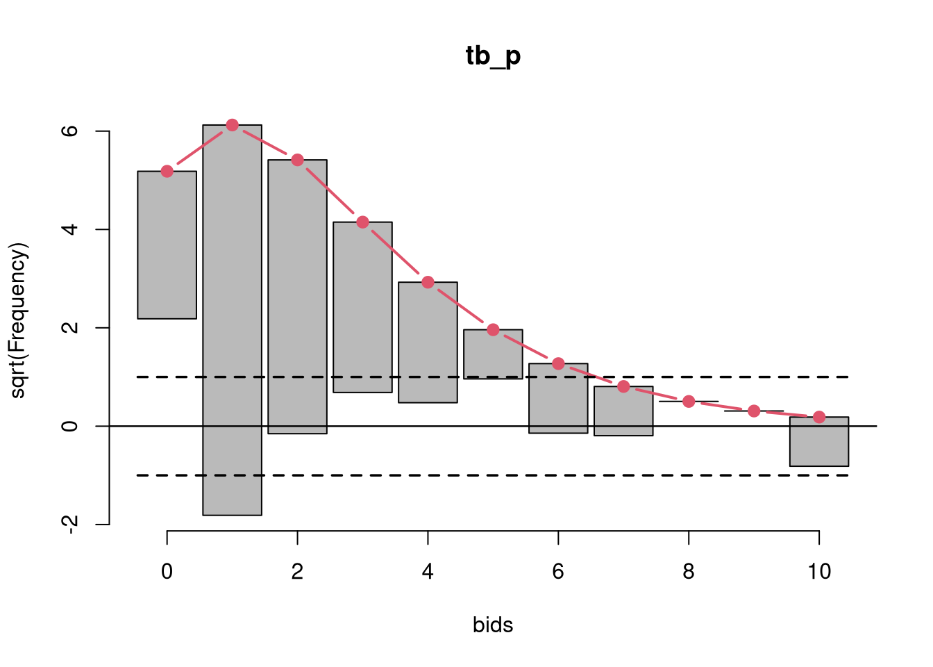
rootogram(tb_p)
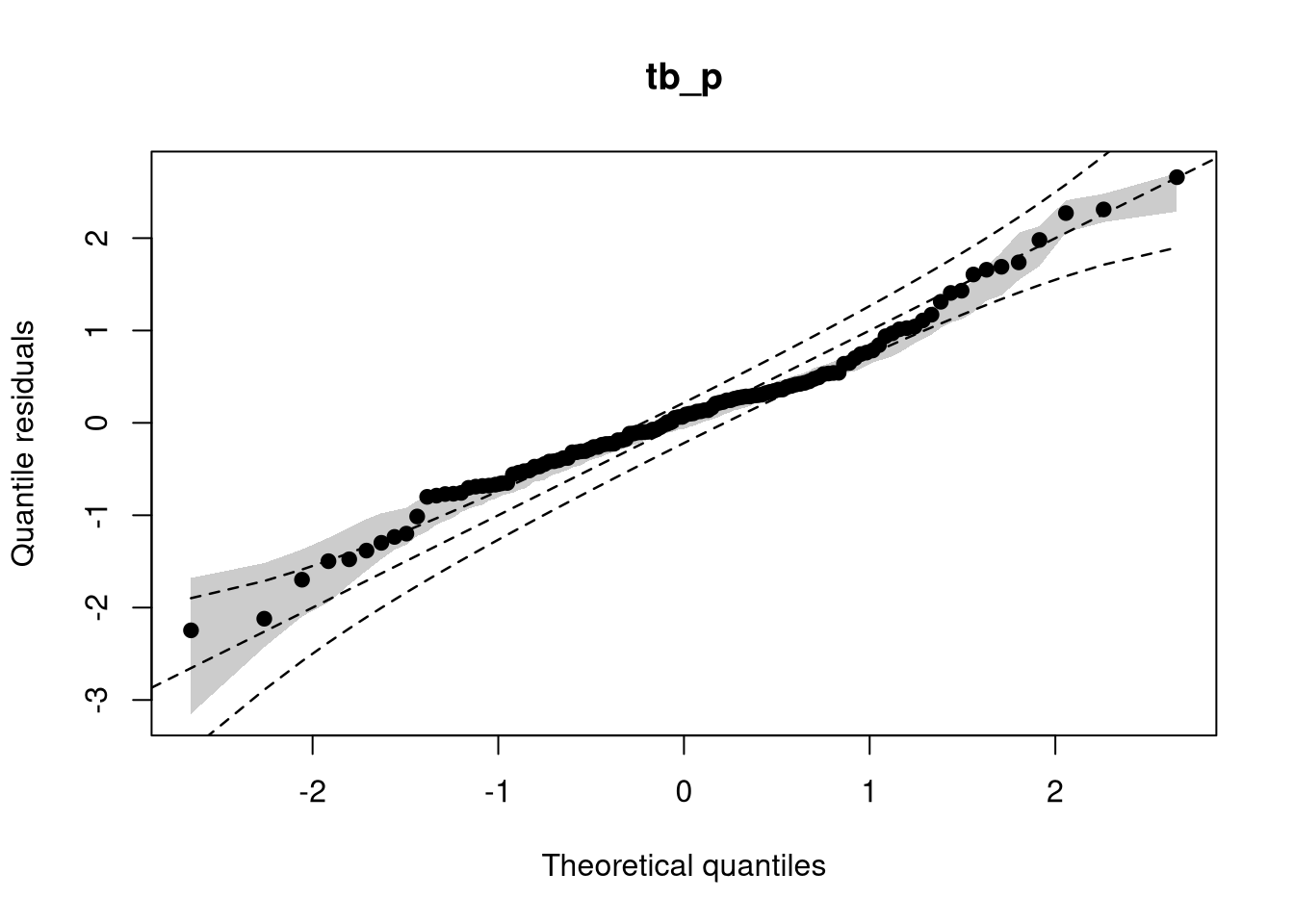
qqrplot(tb_p, range = c(0.05, 0.95))
}

## Parts of Cameron and Trivedi (2013), Table 5.4
summary(residuals(tb_p, type = "response"))

    Min.  1st Qu.   Median     Mean  3rd Qu.     Max. 
-3.22537 -0.71963 -0.07505  0.00000  0.37182  5.57238

summary(residuals(tb_p, type = "pearson"))

     Min.   1st Qu.    Median      Mean   3rd Qu.      Max. 
-1.606458 -0.521439 -0.068443  0.001563  0.297046  3.026831

summary(residuals(tb_p, type = "deviance"))

    Min.  1st Qu.   Median     Mean  3rd Qu.     Max. 
-2.27187 -0.55501 -0.06922 -0.08986  0.28720  2.39771

## hurdle Poisson model mitigates underdispersion
tb_hp <- hurdle(bids ~ . + I(size^2), data = TakeoverBids, dist = "poisson")
AIC(tb_p, tb_hp)

      df      AIC
tb_p  10 389.8967
tb_hp 20 358.9549

if(require("topmodels")) {
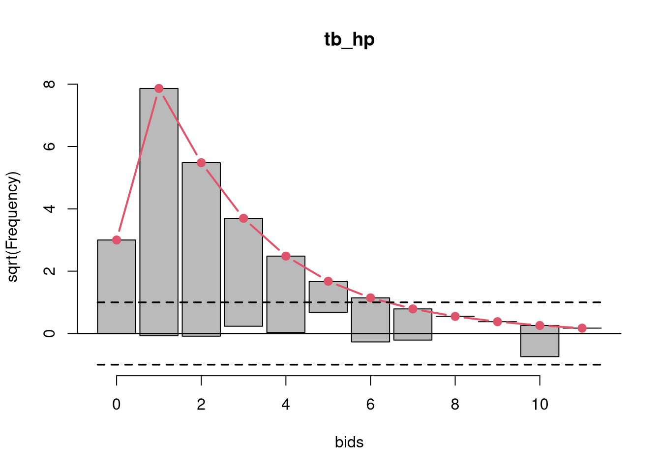
rootogram(tb_hp)
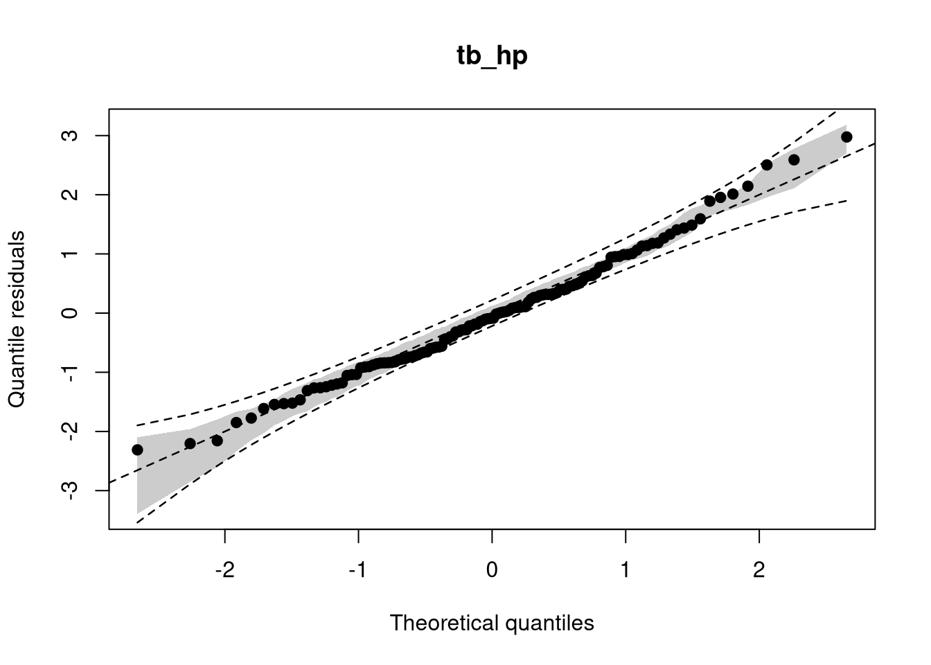
qqrplot(tb_hp, range = c(0.05, 0.95))
}