betareg

Create an Extended-Support Beta Distribution

Description

Class and methods for extended-support beta distributions using the workflow from the distributions3 package.

Usage

XBeta(mu, phi, nu = 0)

Arguments

`mu`	numeric. The mean of the underlying beta distribution on [-nu, 1 + nu].
`phi`	numeric. The precision parameter of the underlying beta distribution on [-nu, 1 + nu].
`nu`	numeric. Exceedence parameter for the support of the underlying beta distribution on [-nu, 1 + nu] that is censored to [0, 1].

Details

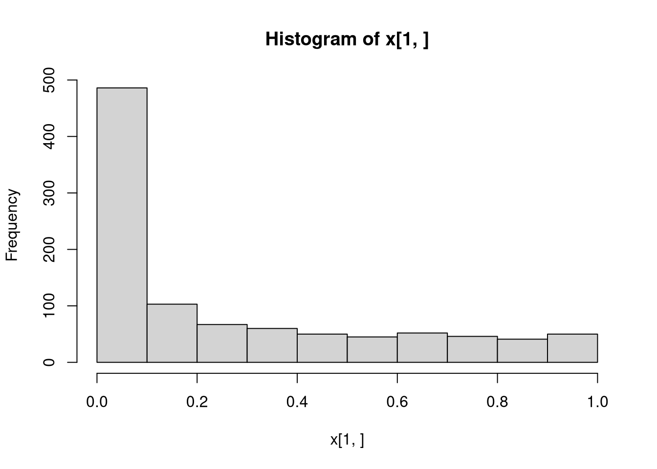
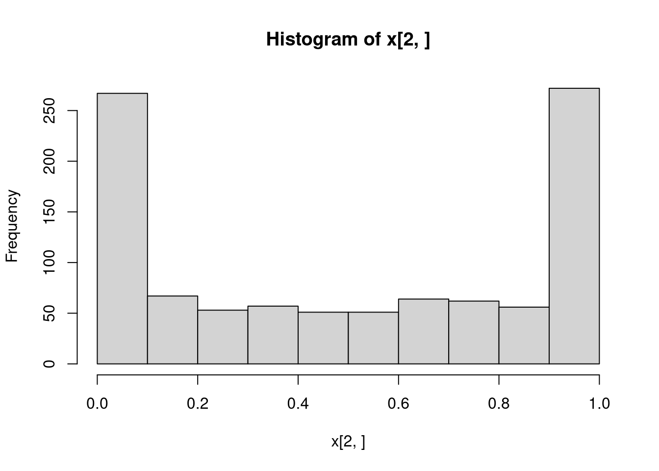
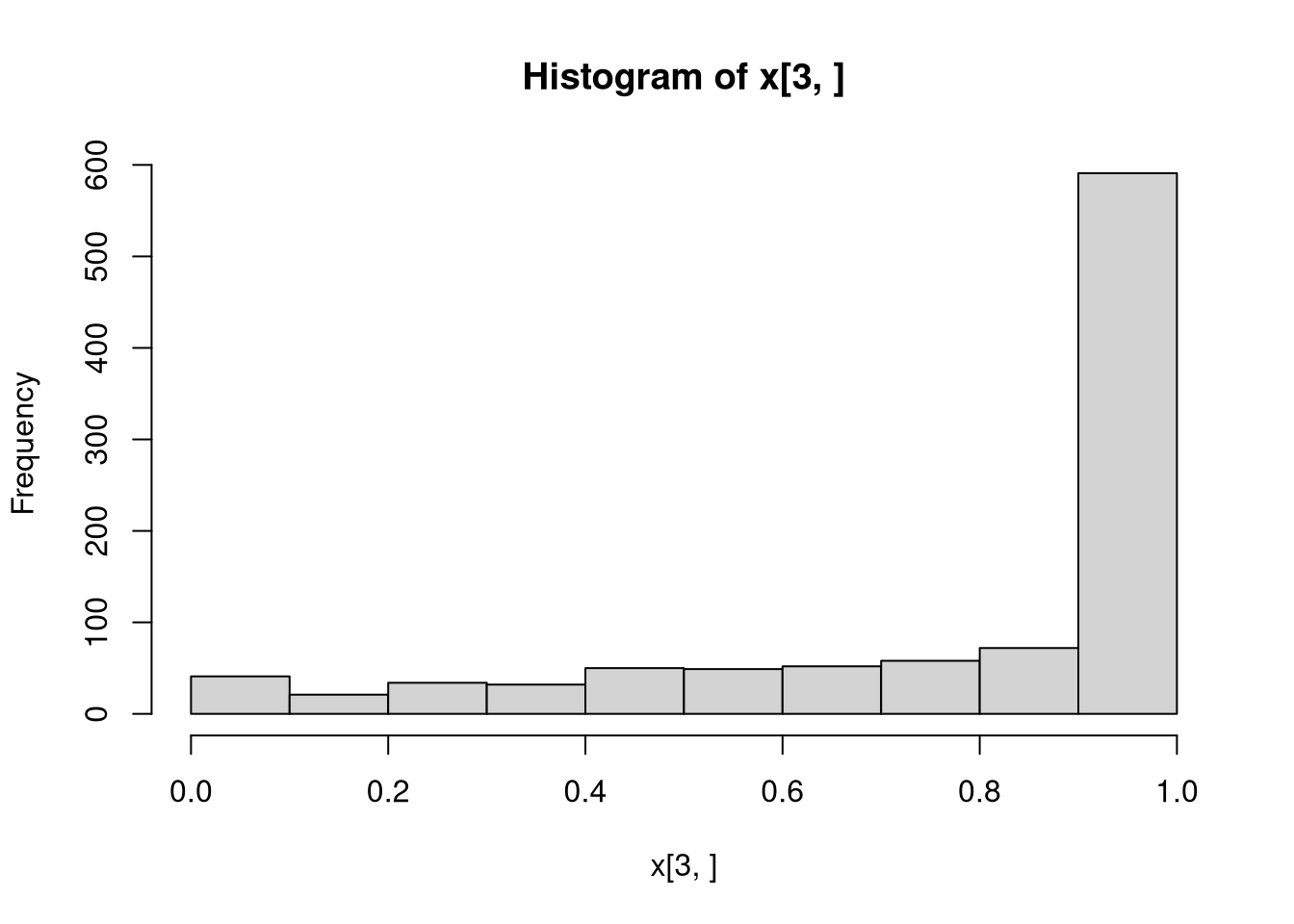
In order to obtain an extended-support beta distribution on [0, 1] an additional exceedence parameter nu is introduced. If nu > 0, this scales the underlying beta distribution to the interval [-nu, 1 + nu] where the tails are subsequently censored to the unit interval [0, 1] with point masses on the boundaries 0 and 1. Thus, nu controls how likely boundary observations are and for nu = 0 (the default), the distribution reduces to the classic beta distribution (in regression parameterization) without boundary observations.

Value

A XBeta distribution object.

Examples

library("betareg")


## package and random seed
library("distributions3")
set.seed(6020)

## three beta distributions
X <- XBeta(
  mu  = c(0.25, 0.50, 0.75),
  phi = c(1, 1, 2),
  nu = c(0, 0.1, 0.2)
)

X

[1] "XBeta(mu = 0.25, phi = 1, nu = 0.0)" "XBeta(mu = 0.50, phi = 1, nu = 0.1)"
[3] "XBeta(mu = 0.75, phi = 2, nu = 0.2)"

## compute moments of the distribution
mean(X)

[1] 0.2500000 0.5000000 0.7886591

variance(X)

[1] 0.09375000 0.15331441 0.08617379

## support interval (minimum and maximum)
support(X)

     min max
[1,]   0   1
[2,]   0   1
[3,]   0   1

## it is only continuous when there are no point masses on the boundary
is_continuous(X)

[1]  TRUE FALSE FALSE

cdf(X, 0)

[1] 0.0000000 0.1864295 0.0239812

cdf(X, 1, lower.tail = FALSE)

[1] 0.0000000 0.1864295 0.4695222

## simulate random variables
random(X, 5)

           r_1       r_2        r_3        r_4       r_5
[1,] 0.7497152 0.8385523 0.03196796 0.91882879 0.5454367
[2,] 0.1263742 1.0000000 0.00000000 0.07151503 0.0000000
[3,] 1.0000000 1.0000000 0.86031184 1.00000000 0.9764434

## histograms of 1,000 simulated observations
x <- random(X, 1000)
hist(x[1, ])

hist(x[2, ])

hist(x[3, ])

## probability density function (PDF) and log-density (or log-likelihood)
x <- c(0.25, 0.5, 0.75)
pdf(X, x)

[1] 0.6840925 0.5305165 0.6607051

pdf(X, x, log = TRUE)

[1] -0.3796622 -0.6339043 -0.4144477

log_pdf(X, x)

[1] -0.3796622 -0.6339043 -0.4144477

## cumulative distribution function (CDF)
cdf(X, x)

[1] 0.6453748 0.5000000 0.3189318

## quantiles
quantile(X, 0.5)

[1] 0.09331223 0.50000000 0.97152842

## cdf() and quantile() are inverses (except at censoring points)
cdf(X, quantile(X, 0.5))

[1] 0.5 0.5 0.5

quantile(X, cdf(X, 1))

[1] 1 1 1

## all methods above can either be applied elementwise or for
## all combinations of X and x, if length(X) = length(x),
## also the result can be assured to be a matrix via drop = FALSE
p <- c(0.05, 0.5, 0.95)
quantile(X, p, elementwise = FALSE)

           q_0.05      q_0.5    q_0.95
[1,] 9.512588e-06 0.09331223 0.9118445
[2,] 0.000000e+00 0.50000000 1.0000000
[3,] 1.199277e-01 0.97152842 1.0000000

quantile(X, p, elementwise = TRUE)

[1] 9.512588e-06 5.000000e-01 1.000000e+00

quantile(X, p, elementwise = TRUE, drop = FALSE)

         quantile
[1,] 9.512588e-06
[2,] 5.000000e-01
[3,] 1.000000e+00

## compare theoretical and empirical mean from 1,000 simulated observations
cbind(
  "theoretical" = mean(X),
  "empirical" = rowMeans(random(X, 1000))
)

     theoretical empirical
[1,]   0.2500000 0.2464581
[2,]   0.5000000 0.4949177
[3,]   0.7886591 0.7955785