Dependency of Anxiety on Stress

Description

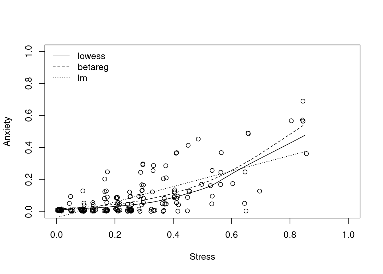
Stress and anxiety among nonclinical women in Townsville, Queensland, Australia.

Usage

data("StressAnxiety", package = "betareg")

Format

A data frame containing 166 observations on 2 variables.

stress

score, linearly transformed to the open unit interval (see below).

anxiety

score, linearly transformed to the open unit interval (see below).

Details

Both variables were assess on the Depression Anxiety Stress Scales, ranging from 0 to 42. Smithson and Verkuilen (2006) transformed these to the open unit interval (without providing details about this transformation).

Source

Example 2 from Smithson and Verkuilen (2006) supplements.

References

Smithson M, Verkuilen J (2006). A Better Lemon Squeezer? Maximum-Likelihood Regression with Beta-Distributed Dependent Variables. Psychological Methods, 11(7), 54–71.

See Also

betareg, MockJurors, ReadingSkills

Examples

library("betareg")

data("StressAnxiety", package = "betareg")
StressAnxiety <- StressAnxiety[order(StressAnxiety$stress),]

## Smithson & Verkuilen (2006, Table 4)
sa_null <- betareg(anxiety ~ 1 | 1,
  data = StressAnxiety, hessian = TRUE)
sa_stress <- betareg(anxiety ~ stress | stress,
  data = StressAnxiety, hessian = TRUE)
summary(sa_null)

Call:
betareg(formula = anxiety ~ 1 | 1, data = StressAnxiety, hessian = TRUE)

Quantile residuals:
    Min      1Q  Median      3Q     Max 
-0.8377 -0.8377 -0.4467  0.6217  3.2396 

Coefficients (mean model with logit link):
            Estimate Std. Error z value Pr(>|z|)    
(Intercept) -2.24396    0.09879  -22.71   <2e-16 ***

Phi coefficients (precision model with log link):
            Estimate Std. Error z value Pr(>|z|)    
(Intercept)    1.796      0.123    14.6   <2e-16 ***
---
Signif. codes:  0 '***' 0.001 '**' 0.01 '*' 0.05 '.' 0.1 ' ' 1 

Type of estimator: ML (maximum likelihood)
Log-likelihood: 239.4 on 2 Df
Number of iterations in BFGS optimization: 9 

summary(sa_stress)

Call:
betareg(formula = anxiety ~ stress | stress, data = StressAnxiety, hessian = TRUE)

Quantile residuals:
    Min      1Q  Median      3Q     Max 
-2.0119 -0.7953 -0.1833  0.5658  3.1141 

Coefficients (mean model with logit link):
            Estimate Std. Error z value Pr(>|z|)    
(Intercept)  -4.0237     0.1442  -27.90   <2e-16 ***
stress        4.9414     0.4409   11.21   <2e-16 ***

Phi coefficients (precision model with log link):
            Estimate Std. Error z value Pr(>|z|)    
(Intercept)   3.9608     0.2511  15.776  < 2e-16 ***
stress       -4.2733     0.7532  -5.674  1.4e-08 ***
---
Signif. codes:  0 '***' 0.001 '**' 0.01 '*' 0.05 '.' 0.1 ' ' 1 

Type of estimator: ML (maximum likelihood)
Log-likelihood:   302 on 4 Df
Pseudo R-squared: 0.4748
Number of iterations in BFGS optimization: 16 

AIC(sa_null, sa_stress)

          df       AIC
sa_null    2 -474.8960
sa_stress  4 -595.9202

1 - as.vector(logLik(sa_null)/logLik(sa_stress))

[1] 0.207021

## visualization
attach(StressAnxiety)
plot(jitter(anxiety) ~ jitter(stress),
  xlab = "Stress", ylab = "Anxiety",
  xlim = c(0, 1), ylim = c(0, 1))
lines(lowess(anxiety ~ stress))
lines(fitted(sa_stress) ~ stress, lty = 2)
lines(fitted(lm(anxiety ~ stress)) ~ stress, lty = 3)
legend("topleft", c("lowess", "betareg", "lm"), lty = 1:3, bty = "n")

detach(StressAnxiety)

## see demo("SmithsonVerkuilen2006", package = "betareg") for more details