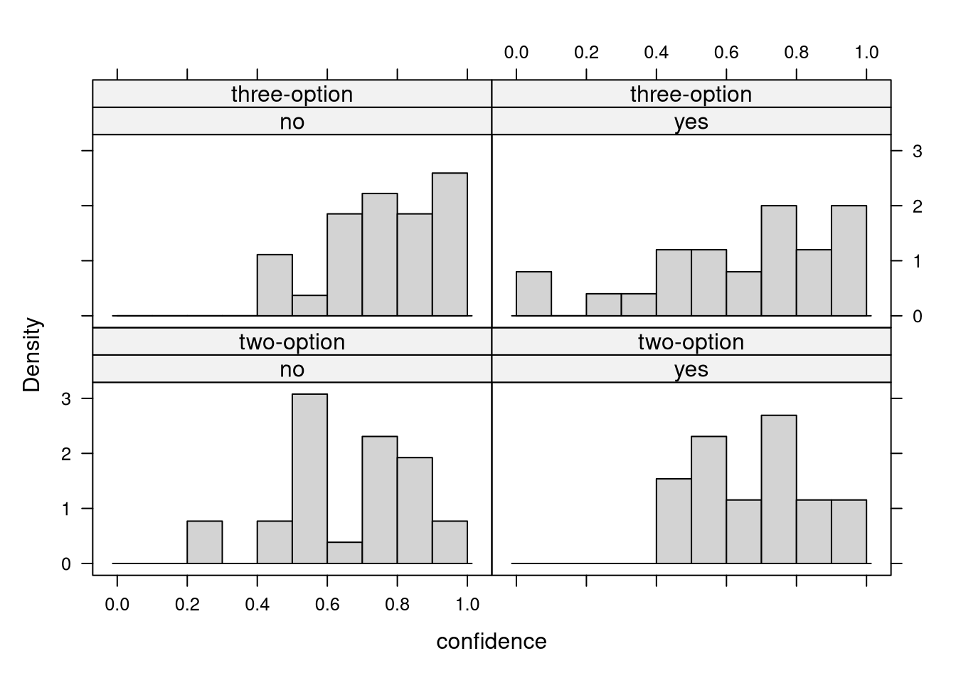
Data with responses of naive mock jurors to the conventional conventional two-option verdict (guilt vs. acquittal) versus a three-option verdict setup (the third option was the Scottish ‘not proven’ alternative), in the presence/absence of conflicting testimonial evidence.
Usage
data("MockJurors", package = "betareg")
Format
A data frame containing 104 observations on 3 variables.
verdict
factor indicating whether a two-option or three-option verdict is requested. (A sum contrast rather than treatment contrast is employed.)
conflict
factor. Is there conflicting testimonial evidence? (A sum contrast rather than treatment contrast is employed.)
confidence
jurors degree of confidence in his/her verdict, scaled to the open unit interval (see below).
Details
The data were collected by Daily (2004) among first-year psychology students at Australian National University. Smithson and Verkuilen (2006) employed the data scaling the original confidence (on a scale 0–100) to the open unit interval: ((original_confidence/100) * 103 - 0.5) / 104.
The original coding of conflict in the data provided from Smithson’s homepage is -1/1 which Smithson and Verkuilen (2006) describe to mean no/yes. However, all their results (sample statistics, histograms, etc.) suggest that it actually means yes/no which was employed in MockJurors.
Source
Example 1 from Smithson and Verkuilen (2006) supplements.
References
Deady S (2004). The Psychological Third Verdict: ‘Not Proven’ or ‘Not Willing to Make a Decision’? Unpublished honors thesis, The Australian National University, Canberra.
Smithson M, Verkuilen J (2006). A Better Lemon Squeezer? Maximum-Likelihood Regression with Beta-Distributed Dependent Variables. Psychological Methods, 11(7), 54–71.
See Also
betareg, ReadingSkills, StressAnxiety
Examples
library("betareg")data("MockJurors", package ="betareg")library("lmtest")## Smithson & Verkuilen (2006, Table 1)## variable dispersion model## (NOTE: numerical rather than analytical Hessian is used for replication,## Smithson & Verkuilen erroneously compute one-sided p-values)mj_vd<-betareg(confidence~verdict*conflict|verdict*conflict, data =MockJurors, hessian =TRUE)summary(mj_vd)
Call:
betareg(formula = confidence ~ verdict * conflict | verdict * conflict,
    data = MockJurors, hessian = TRUE)

Quantile residuals:
    Min      1Q  Median      3Q     Max
-2.4764 -0.6653 -0.0989  0.6000  2.6436

Coefficients (mean model with logit link):
                 Estimate Std. Error z value Pr(>|z|)
(Intercept)      0.912404   0.103979   8.775  < 2e-16 ***
verdict          0.005035   0.103979   0.048  0.96138
conflict         0.168573   0.103979   1.621  0.10497
verdict:conflict 0.280010   0.103979   2.693  0.00708 **

Phi coefficients (precision model with log link):
                 Estimate Std. Error z value Pr(>|z|)
(Intercept)        1.1733     0.1278   9.180  < 2e-16 ***
verdict           -0.3299     0.1278  -2.581  0.00985 **
conflict           0.2196     0.1278   1.718  0.08576 .
verdict:conflict   0.3163     0.1278   2.475  0.01334 *
---
Signif. codes:  0 '***' 0.001 '**' 0.01 '*' 0.05 '.' 0.1 ' ' 1

Type of estimator: ML (maximum likelihood)
Log-likelihood: 40.12 on 8 Df
Pseudo R-squared: 0.03885
Number of iterations in BFGS optimization: 19
## model selection for beta regression: null model, fixed dispersion model (p. 61)mj_null<-betareg(confidence~1|1, data =MockJurors)mj_fd<-betareg(confidence~verdict*conflict|1, data =MockJurors)lrtest(mj_null, mj_fd)
Likelihood ratio test

Model 1: confidence ~ 1 | 1
Model 2: confidence ~ verdict * conflict | 1
  #Df LogLik Df  Chisq Pr(>Chisq)
1   2 28.226
2   5 30.580  3 4.7086     0.1944