truncatednormal

Create a Truncated Normal Distribution

Description

Class and methods for left-, right-, and interval-truncated normal distributions using the workflow from the distributions3 package.

Usage

TruncatedNormal(mu = 0, sigma = 1, left = -Inf, right = Inf)

Arguments

`mu`	numeric. The location parameter of the underlying untruncated normal distribution, typically written \(\mu\) in textbooks. Can be any real number, defaults to `0`.
`sigma`	numeric. The scale parameter (standard deviation) of the underlying untruncated normal distribution, typically written \(\sigma\) in textbooks. Can be any positive number, defaults to `1`.
`left`	numeric. The left truncation point. Can be any real number, defaults to `-Inf` (untruncated). If set to a finite value, the distribution has a point mass at `left` whose probability corresponds to the cumulative probability function of the untruncated normal distribution at this point.
`right`	numeric. The right truncation point. Can be any real number, defaults to `Inf` (untruncated). If set to a finite value, the distribution has a point mass at `right` whose probability corresponds to 1 minus the cumulative probability function of the untruncated normal distribution at this point.

Details

The constructor function TruncatedNormal sets up a distribution object, representing the truncated normal probability distribution by the corresponding parameters: the latent mean mu = \(\mu\) and latent standard deviation sigma = \(\sigma\) (i.e., the parameters of the underlying untruncated normal variable), the left truncation point (with -Inf corresponding to untruncated), and the right truncation point (with Inf corresponding to untruncated).

The truncated normal distribution has probability density function (PDF):

\(f(x) = 1/\sigma \phi((x - \mu)/\sigma) / (\Phi((right - \mu)/\sigma) - \Phi((left - \mu)/\sigma))\)

for \(left \le x \le right\), and 0 otherwise, where \(\Phi\) and \(\phi\) are the cumulative distribution function and probability density function of the standard normal distribution respectively.

All parameters can also be vectors, so that it is possible to define a vector of truncated normal distributions with potentially different parameters. All parameters need to have the same length or must be scalars (i.e., of length 1) which are then recycled to the length of the other parameters.

For the TruncatedNormal distribution objects there is a wide range of standard methods available to the generics provided in the distributions3 package: pdf and log_pdf for the (log-)density (PDF), cdf for the probability from the cumulative distribution function (CDF), quantile for quantiles, random for simulating random variables, crps for the continuous ranked probability score (CRPS), and support for the support interval (minimum and maximum). Internally, these methods rely on the usual d/p/q/r functions provided for the truncated normal distributions in the crch package, see dtnorm, and the crps_tnorm function from the scoringRules package. The methods is_discrete and is_continuous can be used to query whether the distributions are discrete on the entire support (always FALSE) or continuous on the entire support (always TRUE).

See the examples below for an illustration of the workflow for the class and methods.

Value

A TruncatedNormal distribution object.

Examples

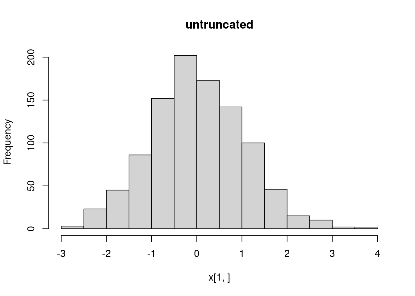
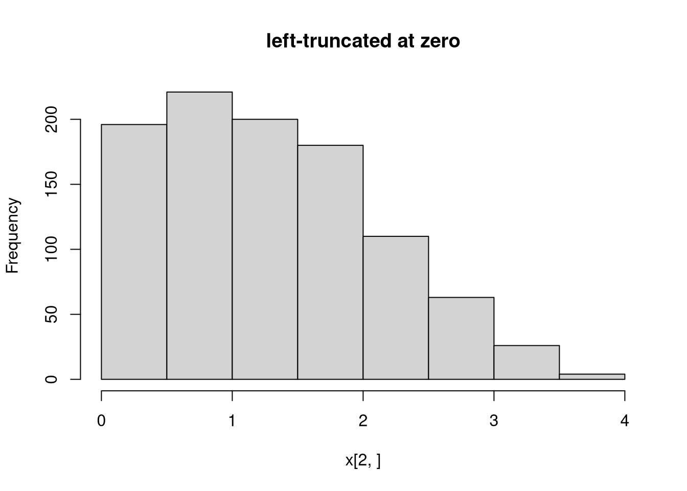
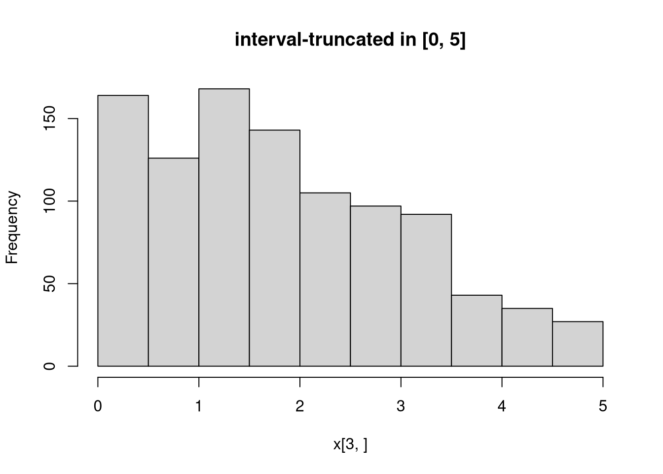
library("crch")


## package and random seed
library("distributions3")
set.seed(6020)

## three truncated normal distributions:
## - untruncated standard normal
## - left-truncated at zero with latent mu = 1 and sigma = 1
## - interval-truncated in [0, 5] with latent mu = 1 and sigma = 2
X <- TruncatedNormal(
  mu    = c(   0,   1, 1),
  sigma = c(   1,   1, 2),
  left  = c(-Inf,   0, 0),
  right = c( Inf, Inf, 5)
)

X

[1] "TruncatedNormal distribution (mu = 0, sigma = 1, left = -Inf, right = Inf)"
[2] "TruncatedNormal distribution (mu = 1, sigma = 1, left =    0, right = Inf)"
[3] "TruncatedNormal distribution (mu = 1, sigma = 2, left =    0, right =   5)"

## compute mean and variance of the truncated distribution
mean(X)

[1] 0.000000 1.287600 1.891488

variance(X)

[1] 1.0000000 0.6296863 1.5063753

## higher moments (skewness, kurtosis) are not implemented yet

## support interval (minimum and maximum)
support(X)

      min max
[1,] -Inf Inf
[2,]    0 Inf
[3,]    0   5

## simulate random variables
random(X, 5)

            r_1       r_2        r_3         r_4         r_5
[1,] -0.3421647 0.4419331 -0.6121245 -0.05869749 -1.74610318
[2,]  0.8831861 1.7520048  1.7872496  0.84989937  0.02234993
[3,]  2.4106941 0.4519601  0.3781711  1.07687138  0.67957521

## histograms of 1,000 simulated observations
x <- random(X, 1000)
hist(x[1, ], main = "untruncated")

hist(x[2, ], main = "left-truncated at zero")

hist(x[3, ], main = "interval-truncated in [0, 5]")

## probability density function (PDF) and log-density (or log-likelihood)
x <- c(0, 0, 1)
pdf(X, x)

[1] 0.3989423 0.2876000 0.2982914

pdf(X, x, log = TRUE)

[1] -0.9189385 -1.2461848 -1.2096844

log_pdf(X, x)

[1] -0.9189385 -1.2461848 -1.2096844

## cumulative distribution function (CDF)
cdf(X, x)

[1] 0.5000000 0.0000000 0.2863151

## quantiles
quantile(X, 0.5)

[1] 0.000000 1.200174 1.732409

## cdf() and quantile() are inverses
cdf(X, quantile(X, 0.5))

[1] 0.5 0.5 0.5

quantile(X, cdf(X, 1))

[1] 1 1 1

## all methods above can either be applied elementwise or for
## all combinations of X and x, if length(X) = length(x),
## also the result can be assured to be a matrix via drop = FALSE
p <- c(0.05, 0.5, 0.95)
quantile(X, p, elementwise = FALSE)

         q_0.05    q_0.5   q_0.95
[1,] -1.6448536 0.000000 1.644854
[2,]  0.1609566 1.200174 2.727185
[3,]  0.1858320 1.732409 4.175247

quantile(X, p, elementwise = TRUE)

[1] -1.644854  1.200174  4.175247

quantile(X, p, elementwise = TRUE, drop = FALSE)

      quantile
[1,] -1.644854
[2,]  1.200174
[3,]  4.175247

## compare theoretical and empirical mean from 1,000 simulated observations
cbind(
  "theoretical" = mean(X),
  "empirical" = rowMeans(random(X, 1000))
)

     theoretical   empirical
[1,]    0.000000 -0.01591685
[2,]    1.287600  1.25873948
[3,]    1.891488  1.90212846

## evaluate continuous ranked probability score (CRPS) using scoringRules
library("scoringRules")
crps(X, x)

[1] 0.2336950 0.8408519 0.4738612