Reliagram (Extended Reliability Diagram)
reliagram.RdReliagram (extended reliability diagram) assess the reliability of a fitted
probabilistic distributional forecast for a binary event. If plot =
TRUE, the resulting object of class "reliagram" is plotted by
plot.reliagram or autoplot.reliagram before it is
returned, depending on whether the package ggplot2 is loaded.
reliagram(object, ...)
# S3 method for default
reliagram(
object,
newdata = NULL,
plot =
TRUE
,
class = NULL,
breaks = seq(0, 1, by = 0.1),
quantiles = 0.5,
thresholds = NULL,
confint = TRUE,
confint_level = 0.95,
confint_nboot = 250,
confint_seed = 1,
single_graph = FALSE,
xlab = "Forecast probability",
ylab = "Observed relative frequency",
main = NULL,
...
)Arguments
- object
an object from which an extended reliability diagram can be extracted with
procast.- ...
further graphical parameters.
- newdata
optionally, a data frame in which to look for variables with which to predict. If omitted, the original observations are used.
- plot
Should the
plotorautoplotmethod be called to draw the computed extended reliability diagram? Either setplotexpicitly to"base"vs."ggplot2"to choose the type of plot, or for a logicalplotargument it's chosen conditional if the packageggplot2is loaded.- class
Should the invisible return value be either a
data.frameor atibble. Either setclassexpicitly to"data.frame"vs."tibble", or forNULLit's chosen automatically conditional if the packagetibbleis loaded.- breaks
numeric vector passed on to
cutin order to bin the observations and the predicted probabilities or a function applied to the predicted probabilities to calculate a numeric value forcut. Typically quantiles to ensure equal number of predictions per bin, e.g., bybreaks = function(x) quantile(x).- quantiles
numeric vector of quantile probabilities with values in [0,1] to calculate single or several thresholds. Only used if
thresholdsis not specified. For binary responses typically the 50%-quantile is used.- thresholds
numeric vector specifying both where to cut the observations into binary values and at which values the predicted probabilities should be calculated (
procast).- confint
logical. Should confident intervals be calculated and drawn?
- confint_level
numeric. The confidence level required.
- confint_nboot
numeric. The number of bootstrap steps.
- confint_seed
numeric. The seed to be set for the bootstrapping.
- single_graph
logical. Should all computed extended reliability diagrams be plotted in a single graph?
- xlab, ylab, main
graphical parameters.
Value
An object of class "reliagram" inheriting from
"data.frame" or "tibble" conditional on the argument class
with the following variables:
- x
forecast probabilities,
- y
observered/empirical relative frequencies,
- bin_lwr, bin_upr
lower and upper bound of the binned forecast probabilities,
- n_pred
number of predictions within the binned forecasts probabilites,
- ci_lwr, ci_upr
lower and upper confidence interval bound.
Additionally,
xlab, ylab, main, and treshold,
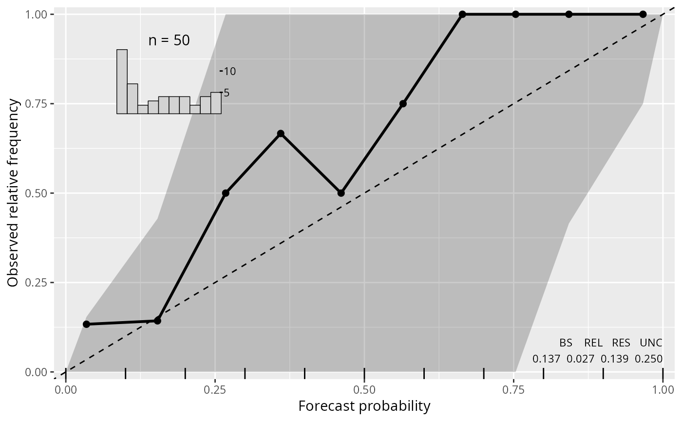
confint_level, as well as the total and the decomposed Brier Score
(bs, rel, res, unc) are stored as attributes.
Details
Reliagrams evaluate if a probability model is calibrated (reliable) by first
partitioning the predicted probability for a binary event into a certain number
of bins and then plotting (within each bin) the averaged forecast probability
against the observered/empirical relative frequency. For computation,
reliagram leverages the procast generic to
forecast the respective predictive probabilities.
For continous probability forecasts, reliability diagrams can be computed either for a pre-specified threshold or for a specific quantile probability of the response values. Per default, reliagrams are computed for the 50%-quantile of the reponse.
In addition to the plot and autoplot method for
reliagram objects, it is also possible to combine two (or more) reliability
diagrams by c/rbind, which creates a set of reliability diagrams
that can then be plotted in one go.
Note
Note that there is also a reliability.plot function in the
verification package. However, it only works for numeric
forecast probabilities and numeric observed relative frequencies, hence a function has been
created here.
References
Wilks DS (2011) Statistical Methods in the Atmospheric Sciences, 3rd ed., Academic Press, 704 pp.
See also
link{plot.reliagram}, procast
Examples
## speed and stopping distances of cars
m1_lm <- lm(dist ~ speed, data = cars)
## compute and plot reliagram
reliagram(m1_lm)
 #-------------------------------------------------------------------------------
## determinants for male satellites to nesting horseshoe crabs
data("CrabSatellites", package = "countreg")
## linear poisson model
m1_pois <- glm(satellites ~ width + color, data = CrabSatellites, family = poisson)
m2_pois <- glm(satellites ~ color, data = CrabSatellites, family = poisson)
## compute and plot reliagram as base graphic
r1 <- reliagram(m1_pois, plot = FALSE)
r2 <- reliagram(m2_pois, plot = FALSE)
## plot combined reliagram as "ggplot2" graphic
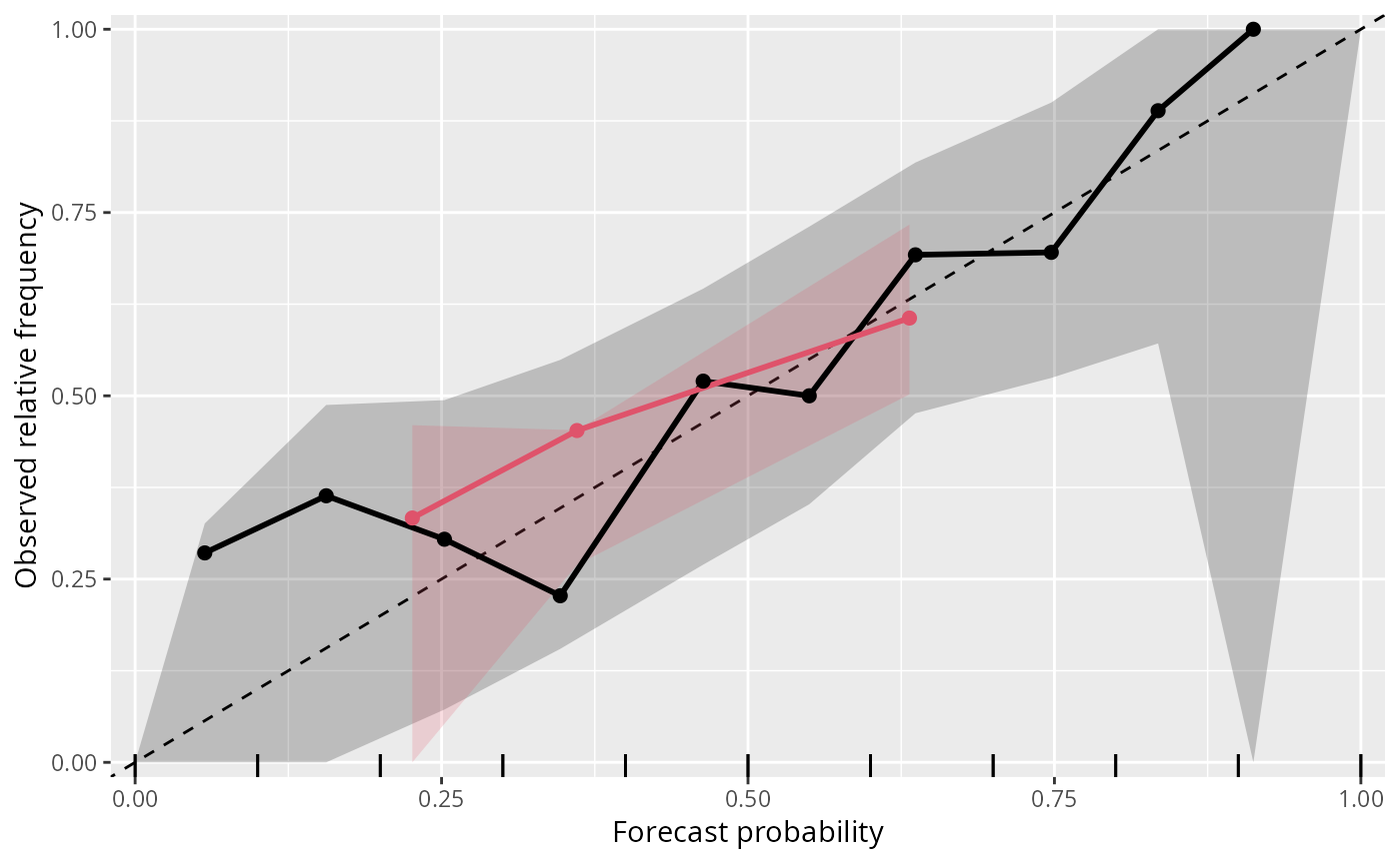
ggplot2::autoplot(c(r1, r2), single_graph = TRUE, col = c(1, 2), fill = c(1, 2))
#-------------------------------------------------------------------------------
## determinants for male satellites to nesting horseshoe crabs
data("CrabSatellites", package = "countreg")
## linear poisson model
m1_pois <- glm(satellites ~ width + color, data = CrabSatellites, family = poisson)
m2_pois <- glm(satellites ~ color, data = CrabSatellites, family = poisson)
## compute and plot reliagram as base graphic
r1 <- reliagram(m1_pois, plot = FALSE)
r2 <- reliagram(m2_pois, plot = FALSE)
## plot combined reliagram as "ggplot2" graphic
ggplot2::autoplot(c(r1, r2), single_graph = TRUE, col = c(1, 2), fill = c(1, 2))