Graphical Model Assessment

Moritz Lang, Achim Zeileis

Artifical data

set.seed(0)

## regressors
d <- data.frame( 
  x = runif(500, -1, 1),
  z = runif(500, -1, 1)
)

## parameters
d <- transform(d,
  lambda = exp(1 + 0.5 * x),
  theta = 2,
  mu = 50 + 22 * x,
  sigma = 22,
  sigmaz = exp(3 + 1 * z)
)

## responses
d <- transform(d,
  ynorm = rnorm(500, mean = mu, sd = sigma),

  yhnorm = rnorm(500, mean = mu, sd = sigmaz),
  ytnorm = crch::rtnorm(500, mean = mu, sd = sigma, left = 0),
  ycnorm = crch::rcnorm(500, mean = mu, sd = sigma, left = 0, right = 100),

  yt = mu + sigma * rt(500, df = 4),
  ylaplace = mu + rmutil::rlaplace(500, s = sigma),
  yrskew = sn::rsn(500, xi = mu, omega = sigma, alpha = 5, tau = 0),
  ylskew = sn::rsn(500, xi = mu, omega = sigma, alpha = -5, tau = 0),
  yunif = mu + sigma * runif(500, min = -1, max = 1),

  ypois = rpois(500, lambda = lambda),
  ynegbin = rnbinom(500, mu = lambda, size = theta),
  yzip = ifelse(runif(500) < 0.25, 0, rpois(500, lambda = lambda))
)

Continuous data

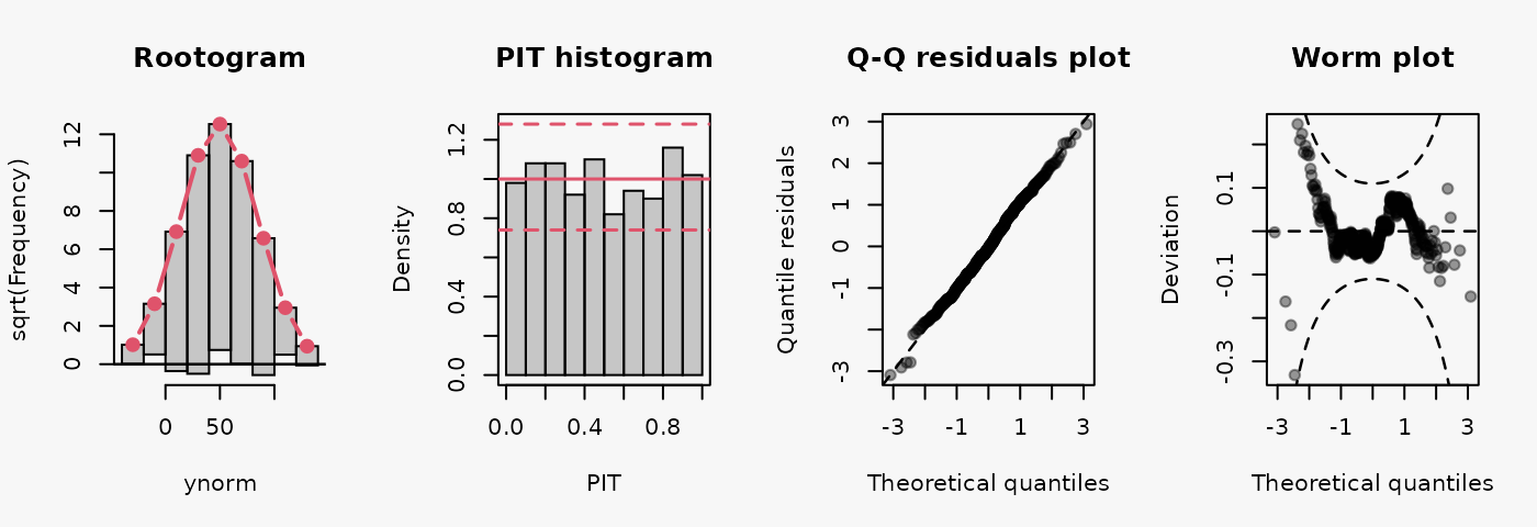
Homoscedastic normal

## correct model fit
m1 <- lm(ynorm ~ x, data = d)

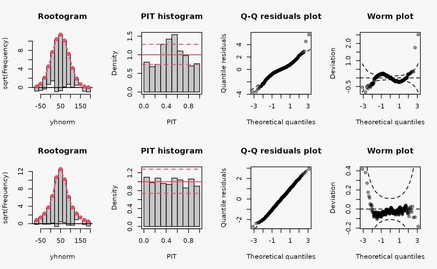
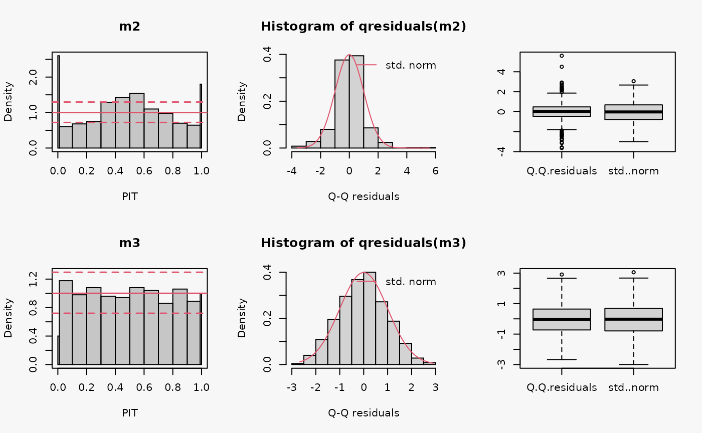
Conditional heteroscedasticity

## not accounting for heteroscedasticity
m2 <- lm(yhnorm ~ x, data = d)

### accounting for heteroscedasticity
m3 <- crch(yhnorm ~ x | z, data = d)

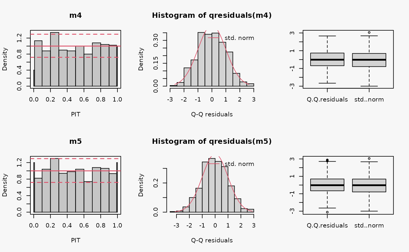
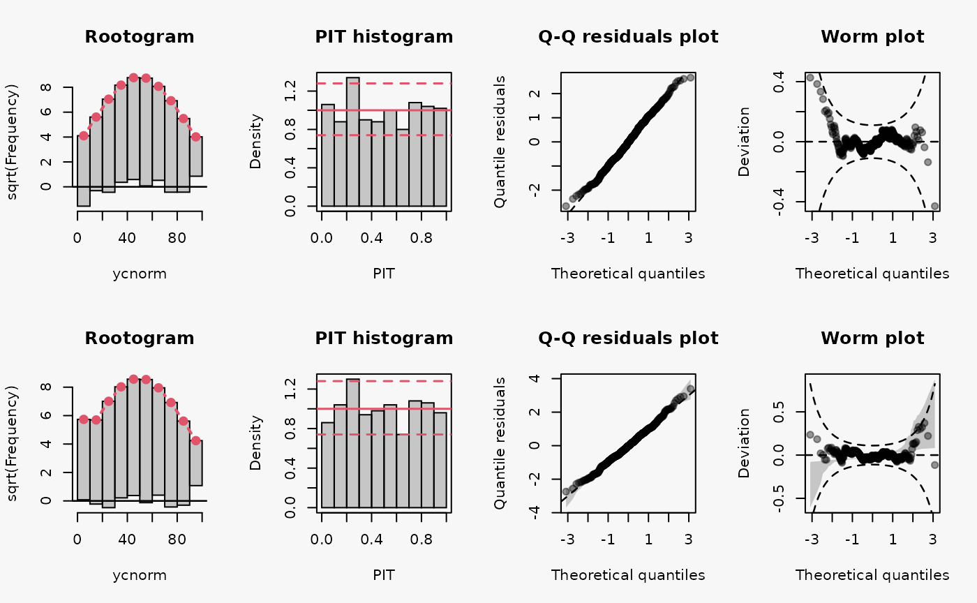
Censoring (0, 100)

## not accounting for censoring
m4 <- lm(ycnorm ~ x, data = d)

## accounting for censoring
m5 <- crch(ycnorm ~ x | 1, data = d, left = 0, right = 100)

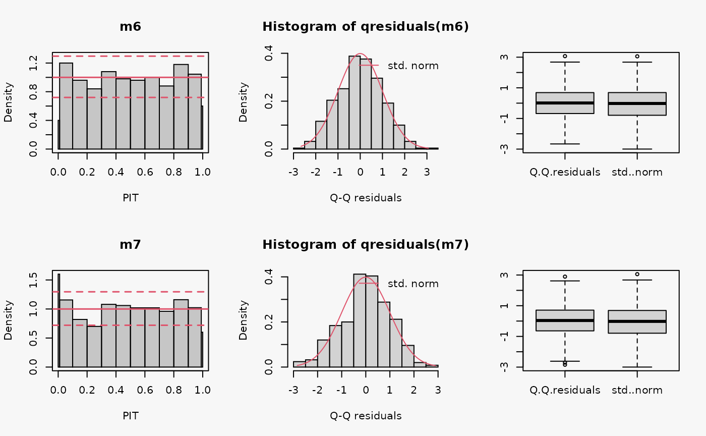
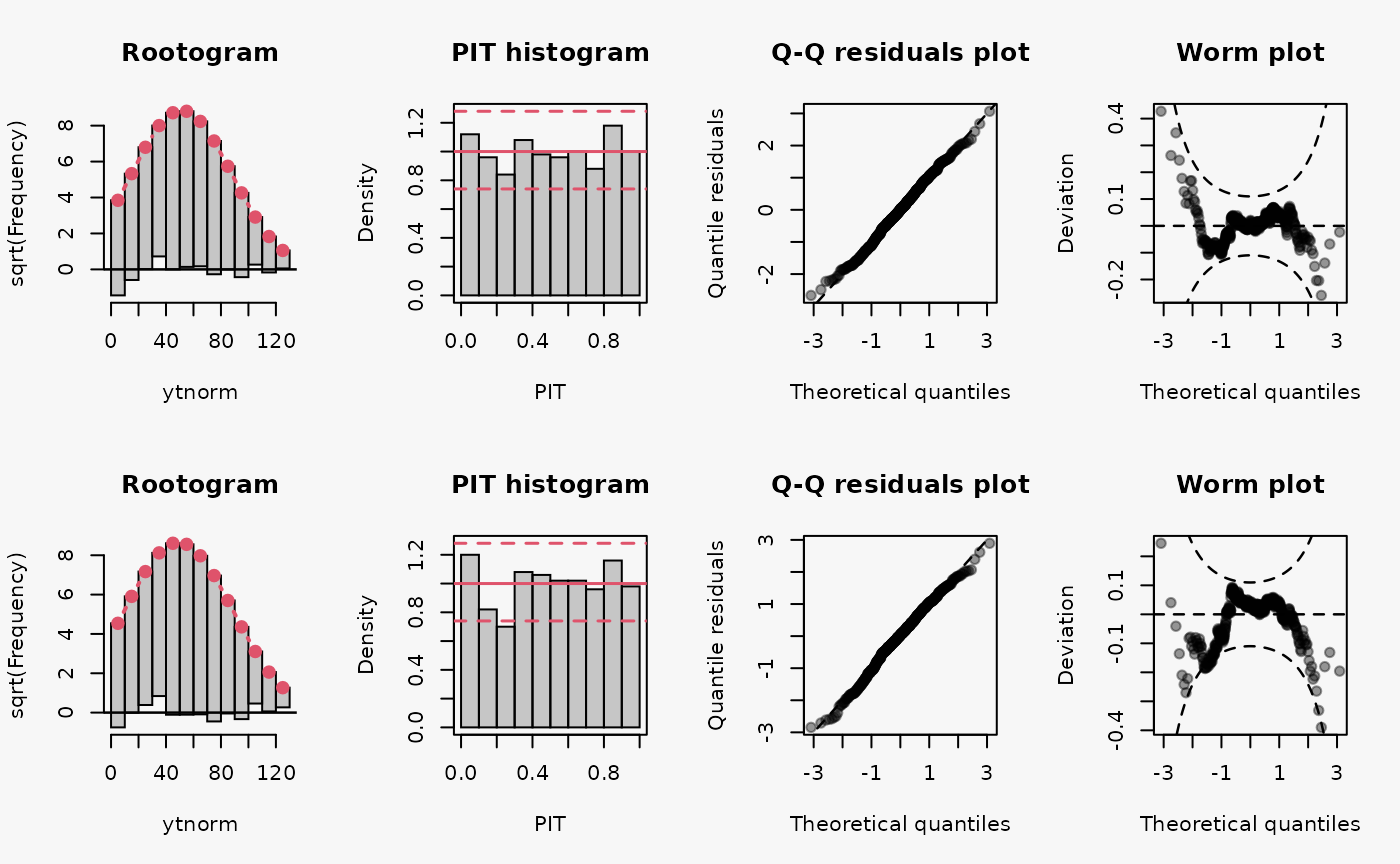
Truncation (> 0)

## not accounting for truncation
m6 <- lm(ytnorm ~ x, data = d)

# not accounting for truncation
m7 <- trch(ytnorm ~ x | 1, data = d, left = 0)

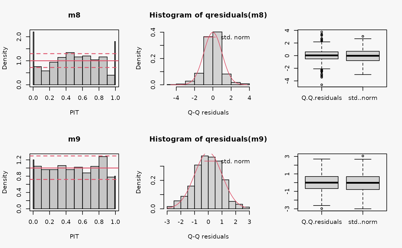
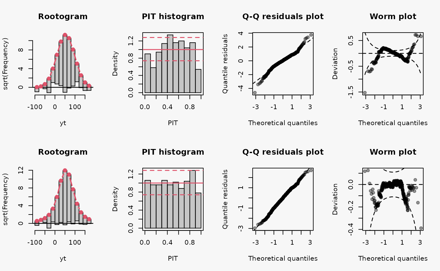
Heavy tails (t_4)

## not accounting for heavy tails
m8 <- lm(yt ~ x, data = d)

## accounting for heavy tails
m9 <- crch(yt ~ x | 1, data = d, dist = "student")

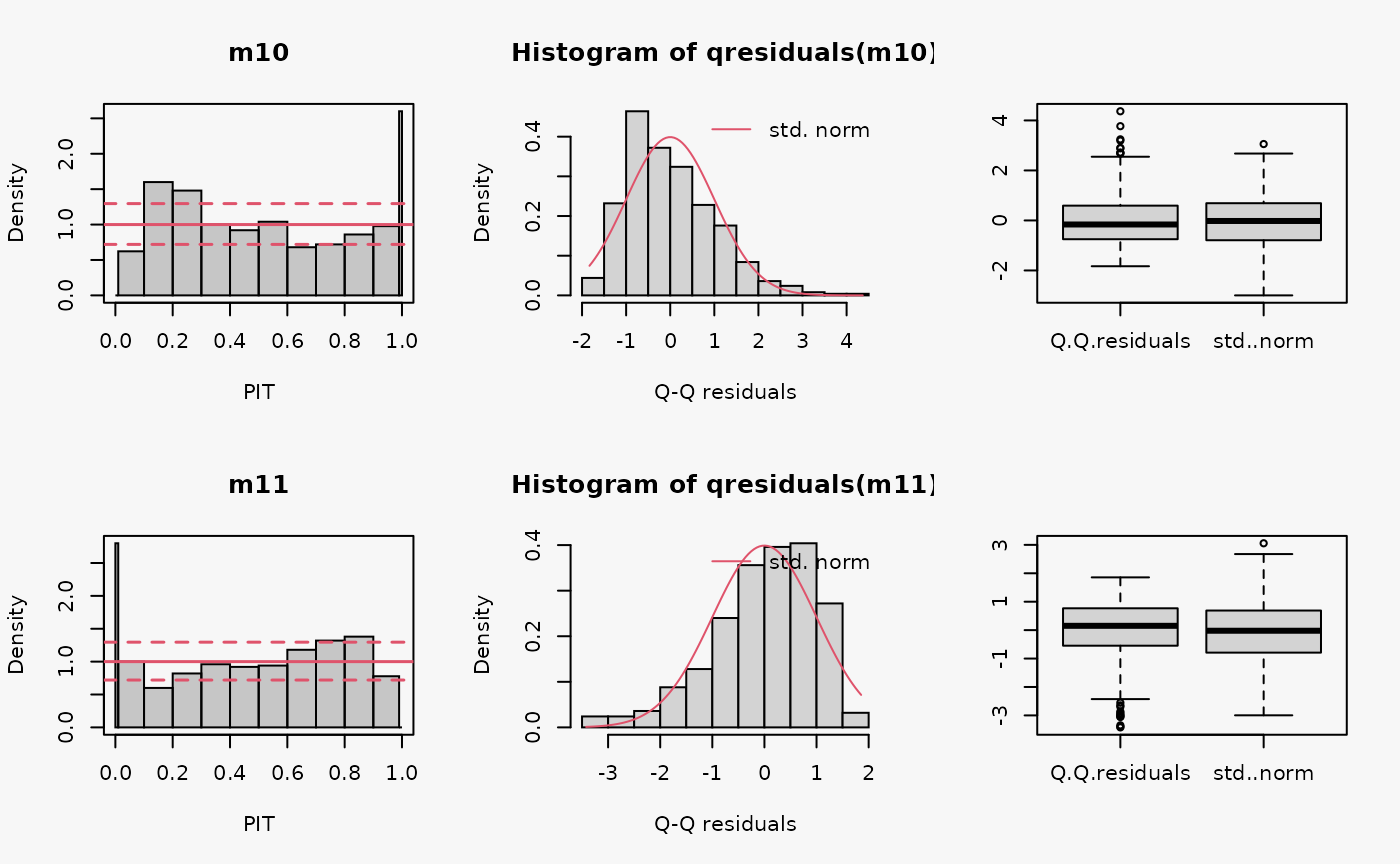
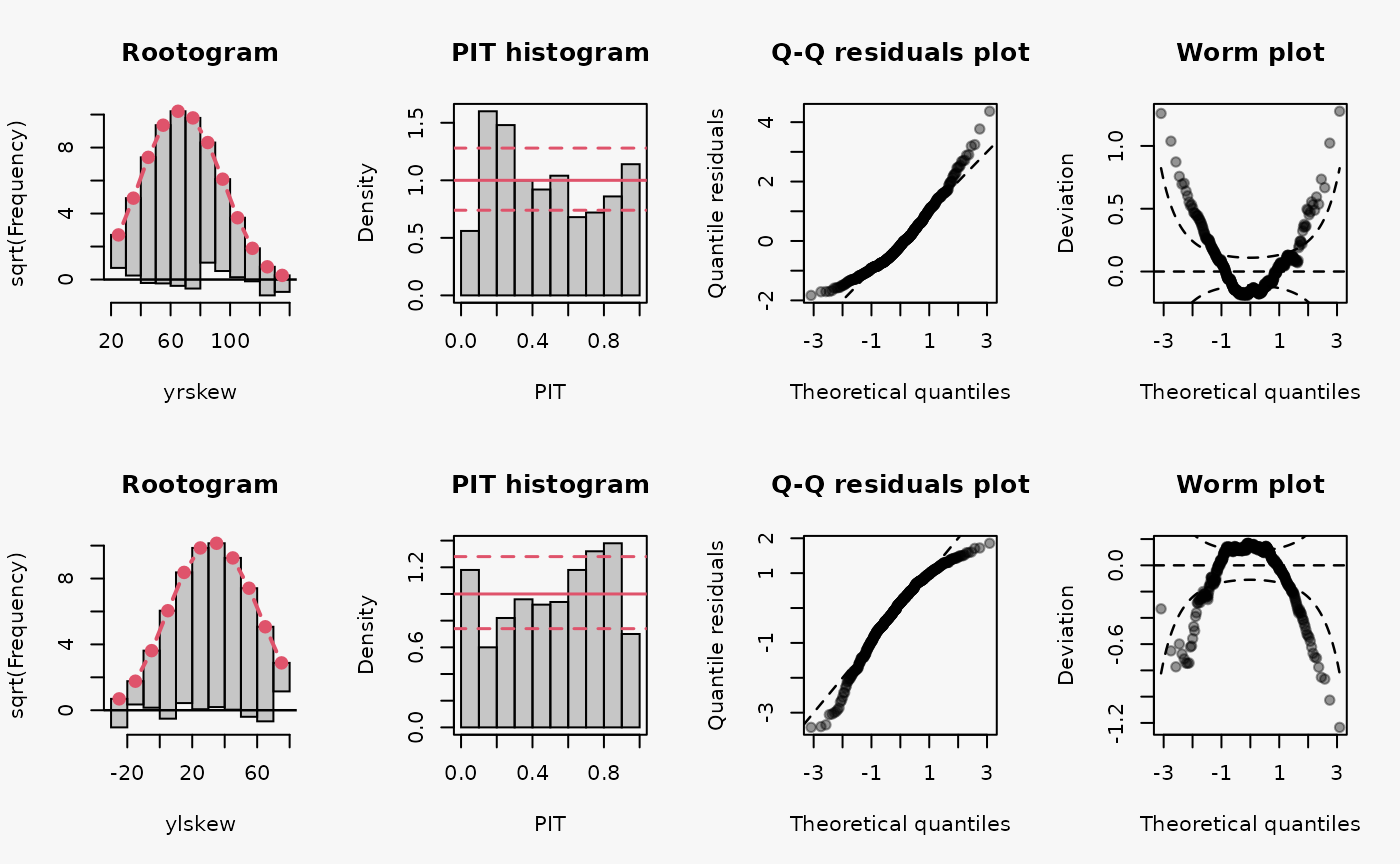
Skewness

## not accounting for right skewed residuals
m10 <- lm(yrskew ~ x, data = d)

## not accounting for left skewed residuals
m11 <- lm(ylskew ~ x, data = d)

Over-/Underdispersion

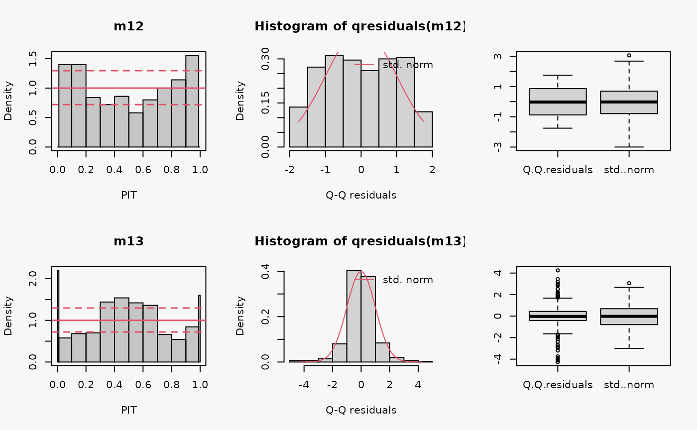
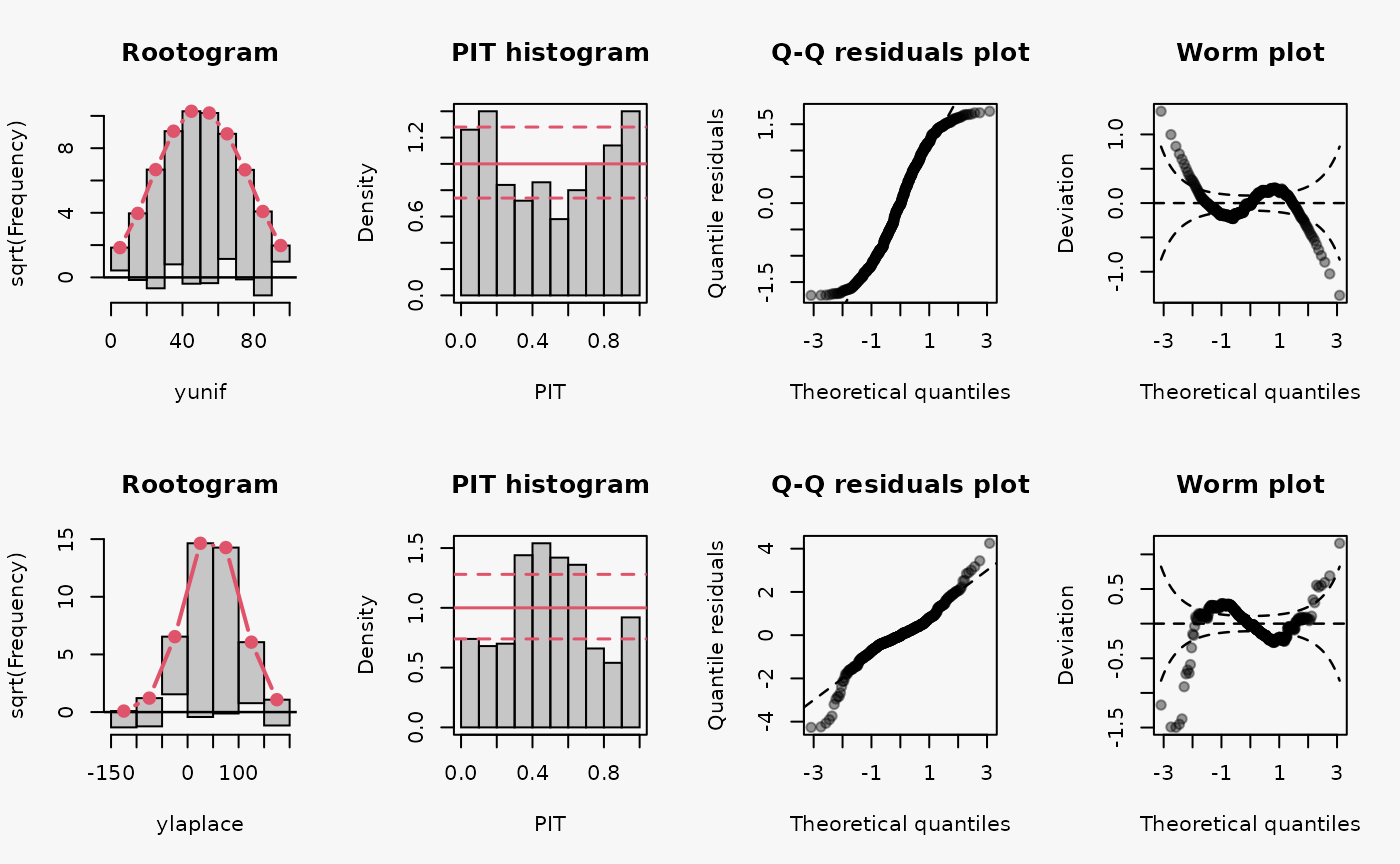
Other misspecified distribution: uniform, laplace

## misspecified distribution leading to an underdispersed predictive distribution
m12 <- lm(yunif ~ x, data = d)

## misspecified distribution leading to an overdispersed predictive distribution
m13 <- lm(ylaplace ~ x, data = d)

Count data

Poisson

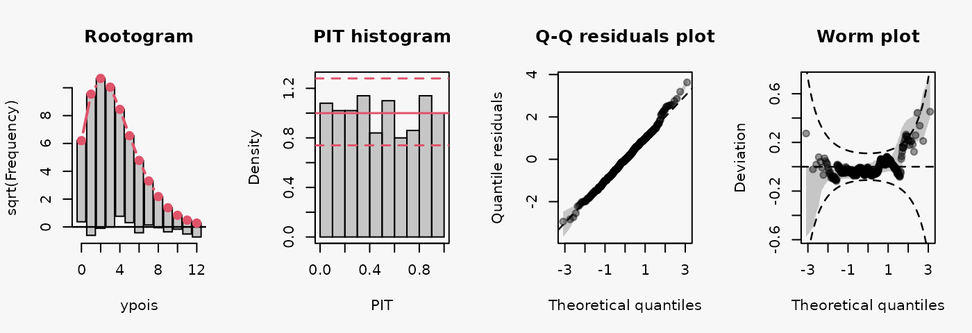
## correct model fit
cm1 <- glm(ypois ~ x, data = d, family = poisson)

Overdispersion (negative binomial)

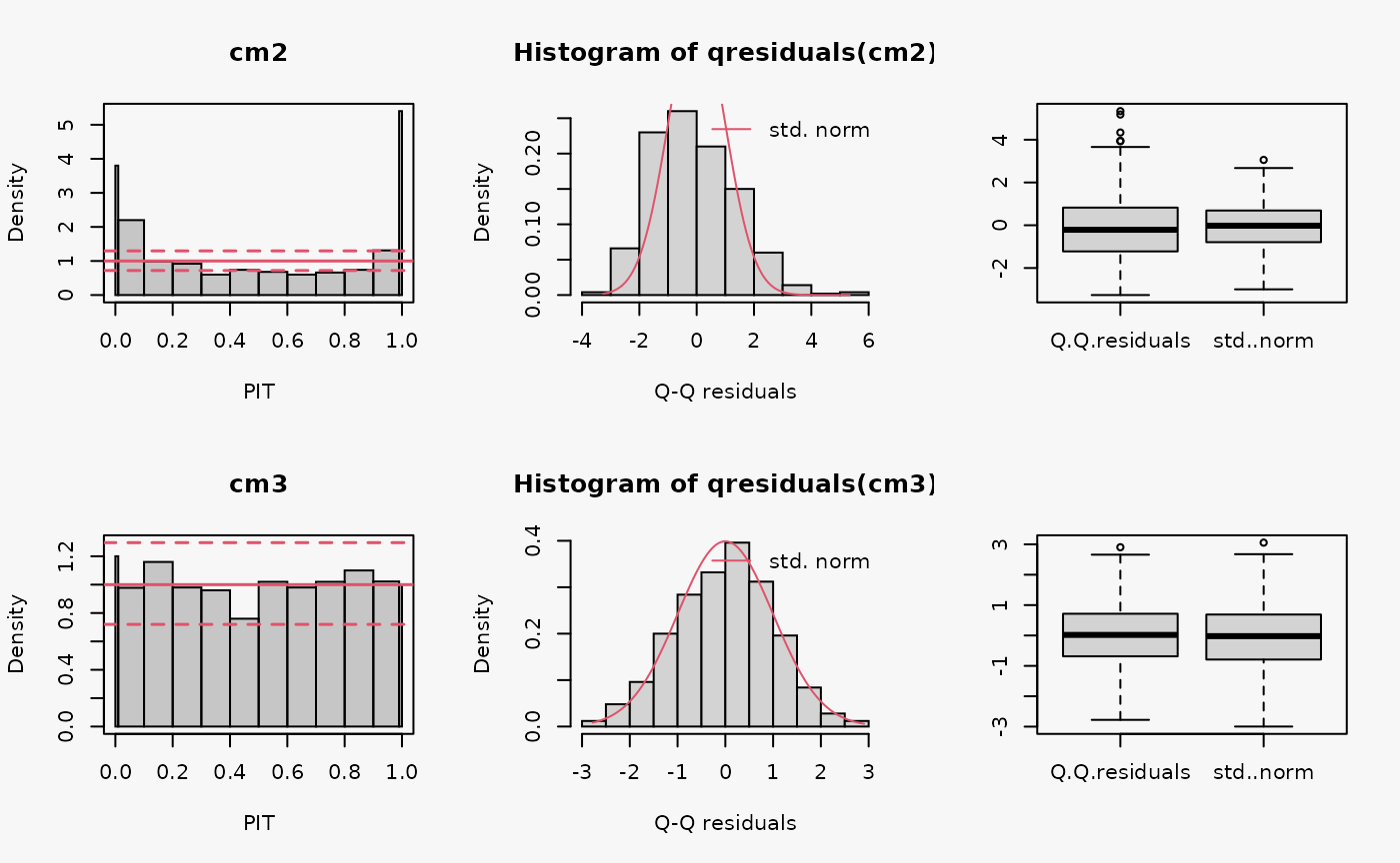
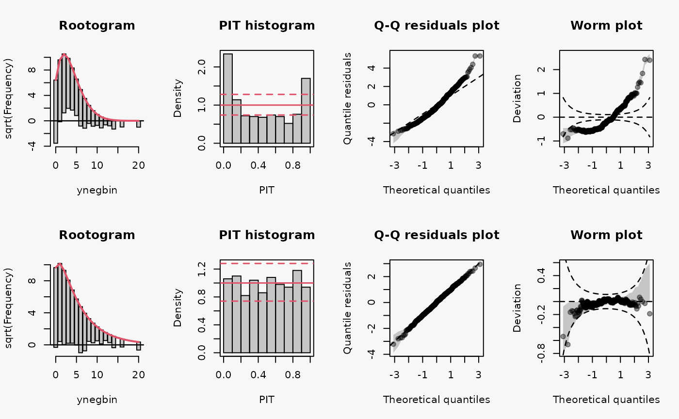
## misspecified distribution leading to an overdispersed predictive distribution
cm2 <- glm(ynegbin ~ x, data = d, family = poisson)

## correct distributional assumption
cm3 <- MASS::glm.nb(ynegbin ~ x, data = d)

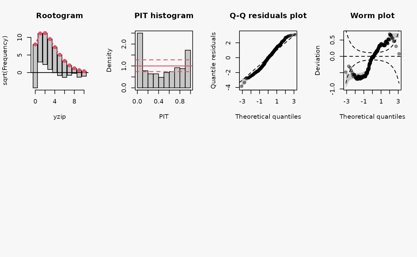
Zero-inflation

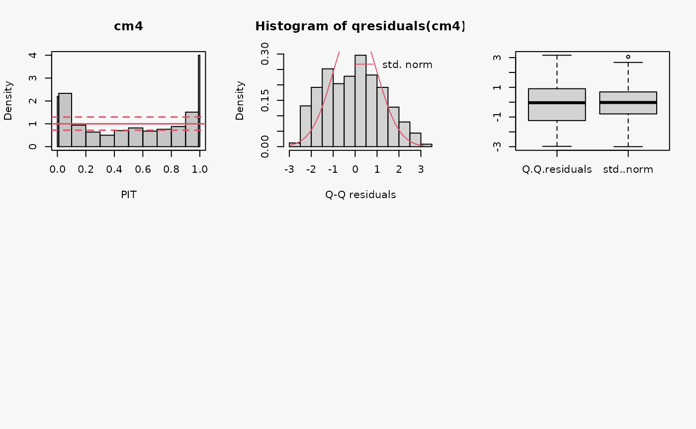
## not accouting for zero inflation
cm4 <- glm(yzip ~ x, data = d, family = poisson)

## accouting for zero inflation
cm5 <- pscl::zeroinfl(yzip ~ x | 1, data = d, dist = "poisson")

Summary

Graph	Calibrated	Right skewed	Left skewed	Underdispersed
Rootogram	-	-	-	-
PIT histogram	Uniform	-	-	U-shape
Q-Q residuals plot	Straightline	-	-	S-shape
Worm plot	Uniform	-	-	-

References