S3 Methods for Plotting Rootograms

Generic plotting functions for rootograms of the class "rootogram" computed by link{rootogram}.

# S3 method for rootogram
plot(
  x,
  style = NULL,
  scale = NULL,
  expected = NULL,
  ref = NULL,
  confint = NULL,
  confint_level = 0.95,
  confint_type = c("pointwise", "simultaneous"),
  confint_nrep = 1000,
  xlim = c(NA, NA),
  ylim = c(NA, NA),
  xlab = NULL,
  ylab = NULL,
  main = NULL,
  axes = TRUE,
  box = FALSE,
  col = "darkgray",
  border = "black",
  lwd = 1,
  lty = 1,
  alpha_min = 0.8,
  expected_col = 2,
  expected_pch = 19,
  expected_lty = 1,
  expected_lwd = 2,
  confint_col = "black",
  confint_lty = 2,
  confint_lwd = 1.75,
  ref_col = "black",
  ref_lty = 1,
  ref_lwd = 1.25,
  ...
)

# S3 method for rootogram
autoplot(
  object,
  style = NULL,
  scale = NULL,
  expected = NULL,
  ref = NULL,
  confint = NULL,
  confint_level = 0.95,
  confint_type = c("pointwise", "simultaneous"),
  confint_nrep = 1000,
  xlim = c(NA, NA),
  ylim = c(NA, NA),
  xlab = NULL,
  ylab = NULL,
  main = NULL,
  legend = FALSE,
  theme = NULL,
  colour = "black",
  fill = "darkgray",
  size = 0.5,
  linetype = 1,
  alpha = NA,
  expected_colour = 2,
  expected_size = 1,
  expected_linetype = 1,
  expected_alpha = 1,
  expected_fill = NA,
  expected_stroke = 0.5,
  expected_shape = 19,
  confint_colour = "black",
  confint_size = 0.5,
  confint_linetype = 2,
  confint_alpha = NA,
  ref_colour = "black",
  ref_size = 0.5,
  ref_linetype = 1,
  ref_alpha = NA,
  ...
)

Arguments

x, object

an object of class rootogram.

style

character specifying the syle of rootogram.

scale

character specifying whether raw frequencies or their square roots (default) should be drawn.

expected

Should the expected (fitted) frequencies be plotted?

ref

logical. Should a reference line be plotted?

confint

logical. Should confident intervals be drawn?

confint_level

numeric. The confidence level required.

confint_type

character. Should "pointwise" or "simultaneous" confidence intervals be visualized.

confint_nrep

numeric. The repetition number of simulation for computing the confidence intervals.

xlim, ylim, xlab, ylab, main, axes, box

graphical parameters.

col, border, lwd, lty, alpha_min

graphical parameters for the histogram style part of the base plot.

expected_col, expected_pch, expected_lty, expected_lwd, ref_col, ref_lty, ref_lwd, expected_colour, expected_size, expected_linetype, expected_alpha, expected_fill, expected_stroke, expected_shape, ref_colour, ref_size, ref_linetype, ref_alpha, confint_col, confint_lty, confint_lwd, confint_colour, confint_size, confint_linetype, confint_alpha

Further graphical parameters for the `expected` and `ref` line using either autoplot or plot.

...

further graphical parameters passed to the plotting function.

legend

logical. Should a legend be added in the ggplot2 style graphic?

theme

Which `ggplot2` theme should be used. If not set, theme_bw is employed.

colour, fill, size, linetype, alpha

graphical parameters for the histogram style part in the autoplot.

Details

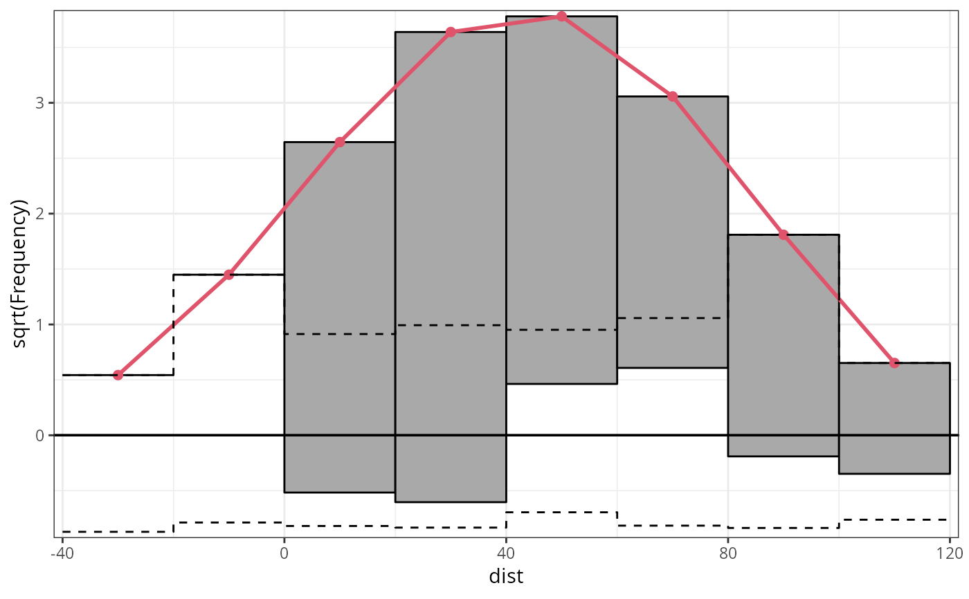
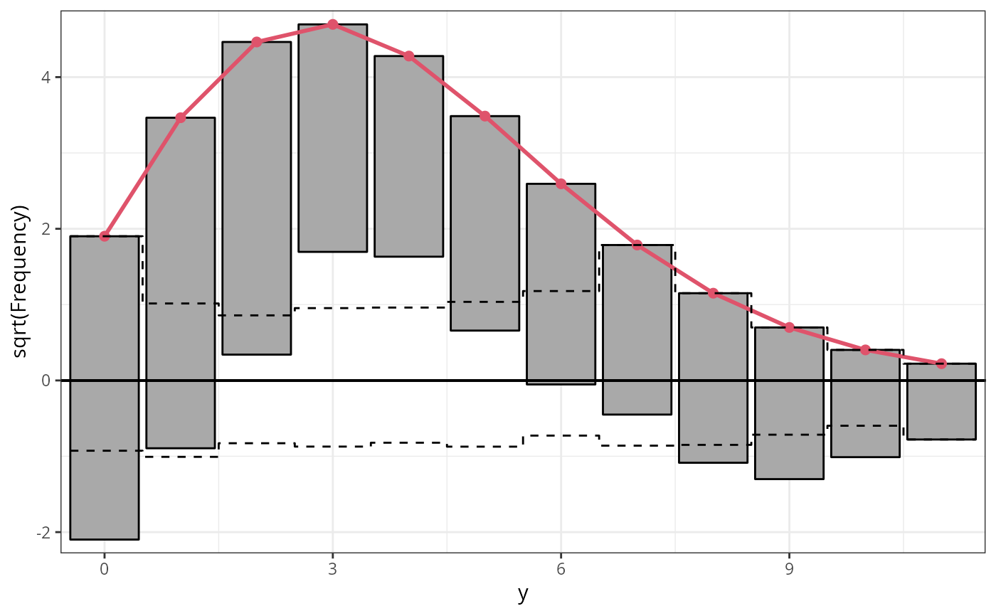
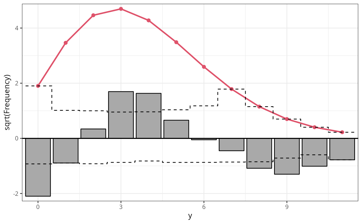
Rootograms graphically compare (square roots) of empirical frequencies with expected (fitted) frequencies from a probability model.

Rootograms graphically compare frequencies of empirical distributions and expected (fitted) probability models. For the observed distribution the histogram is drawn on a square root scale (hence the name) and superimposed with a line for the expected frequencies. The histogram can be "standing" on the x-axis (as usual), or "hanging" from the expected (fitted) curve, or a "suspended" histogram of deviations can be drawn.

References

Friendly M (2000), Visualizing Categorical Data. SAS Institute, Cary.

Kleiber C, Zeileis A (2016). “Visualizing Count Data Regressions Using Rootograms.” The American Statistician, 70(3), 296--303. c("\Sexpr[results=rd,stage=build]tools:::Rd_expr_doi(\"#1\")", "10.1080/00031305.2016.1173590")doi:10.1080/00031305.2016.1173590 .

Tukey JW (1977). Exploratory Data Analysis. Addison-Wesley, Reading.

See also

rootogram, procast

Examples

## speed and stopping distances of cars
m1_lm <- lm(dist ~ speed, data = cars)

## compute and plot rootogram
rootogram(m1_lm)


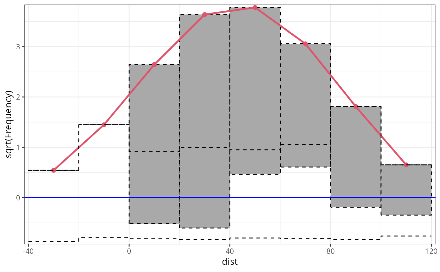
## customize colors
rootogram(m1_lm, ref_col = "blue", lty = 2, pch = 20)


#-------------------------------------------------------------------------------
if (require("crch")) {

  ## precipitation observations and forecasts for Innsbruck
  data("RainIbk", package = "crch")
  RainIbk <- sqrt(RainIbk)
  RainIbk$ensmean <- apply(RainIbk[, grep("^rainfc", names(RainIbk))], 1, mean)
  RainIbk$enssd <- apply(RainIbk[, grep("^rainfc", names(RainIbk))], 1, sd)
  RainIbk <- subset(RainIbk, enssd > 0)

  ## linear model w/ constant variance estimation
  m2_lm <- lm(rain ~ ensmean, data = RainIbk)

  ## logistic censored model
  m2_crch <- crch(rain ~ ensmean | log(enssd), data = RainIbk, left = 0, dist = "logistic")

  ### compute rootograms FIXME
  #r2_lm <- rootogram(m2_lm, plot = FALSE)
  #r2_crch <- rootogram(m2_crch, plot = FALSE)

  ### plot in single graph
  #plot(c(r2_lm, r2_crch), col = c(1, 2))
}

#-------------------------------------------------------------------------------
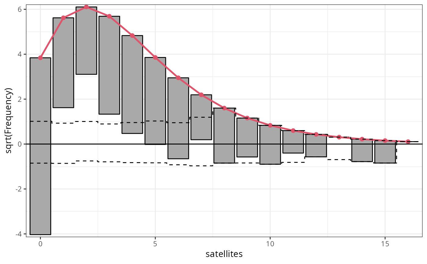
## determinants for male satellites to nesting horseshoe crabs
data("CrabSatellites", package = "countreg")

## linear poisson model
m3_pois <- glm(satellites ~ width + color, data = CrabSatellites, family = poisson)

## compute and plot rootogram as "ggplot2" graphic
rootogram(m3_pois, plot = "ggplot2")


#-------------------------------------------------------------------------------
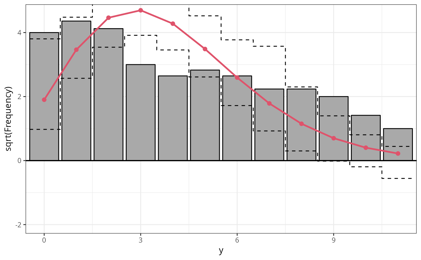
## artificial data from negative binomial (mu = 3, theta = 2)
## and Poisson (mu = 3) distribution
set.seed(1090)
y <- rnbinom(100, mu = 3, size = 2)
x <- rpois(100, lambda = 3)

## glm method: fitted values via glm()
m4_pois <- glm(y ~ x, family = poisson)

## correctly specified Poisson model fit
par(mfrow = c(1, 3))
r4a_pois <- rootogram(m4_pois, style = "standing", ylim = c(-2.2, 4.8), main = "Standing")

r4b_pois <- rootogram(m4_pois, style = "hanging", ylim = c(-2.2, 4.8), main = "Hanging")

r4c_pois <- rootogram(m4_pois, style = "suspended", ylim = c(-2.2, 4.8), main = "Suspended")

par(mfrow = c(1, 1))