S3 Methods for Plotting Q-Q Residuals Plots

Generic plotting functions for Q-Q residual plots for objects of class "qqrplot" returned by link{qqrplot}.

# S3 method for qqrplot
plot(
  x,
  single_graph = FALSE,
  detrend = NULL,
  simint = NULL,
  confint = NULL,
  confint_type = c("pointwise", "simultaneous", "tail-sensitive"),
  confint_level = 0.95,
  ref = NULL,
  ref_identity = TRUE,
  ref_probs = c(0.25, 0.75),
  xlim = c(NA, NA),
  ylim = c(NA, NA),
  xlab = NULL,
  ylab = NULL,
  main = NULL,
  axes = TRUE,
  box = TRUE,
  col = "black",
  pch = 19,
  simint_col = "black",
  simint_alpha = 0.2,
  confint_col = "black",
  confint_lty = 2,
  confint_lwd = 1.25,
  confint_alpha = NULL,
  ref_col = "black",
  ref_lty = 2,
  ref_lwd = 1.25,
  ...
)

# S3 method for qqrplot
points(
  x,
  detrend = NULL,
  simint = FALSE,
  col = "black",
  pch = 19,
  simint_col = "black",
  simint_alpha = 0.2,
  ...
)

# S3 method for qqrplot
autoplot(
  object,
  single_graph = FALSE,
  detrend = NULL,
  simint = NULL,
  confint = NULL,
  confint_type = c("pointwise", "simultaneous", "tail-sensitive"),
  confint_level = 0.95,
  ref = NULL,
  ref_identity = TRUE,
  ref_probs = c(0.25, 0.75),
  xlim = c(NA, NA),
  ylim = c(NA, NA),
  xlab = NULL,
  ylab = NULL,
  main = NULL,
  legend = FALSE,
  theme = NULL,
  alpha = NA,
  colour = "black",
  fill = NA,
  shape = 19,
  size = 2,
  stroke = 0.5,
  simint_fill = "black",
  simint_alpha = 0.2,
  confint_colour = NULL,
  confint_fill = NULL,
  confint_size = NULL,
  confint_linetype = NULL,
  confint_alpha = NULL,
  ref_colour = "black",
  ref_size = 0.5,
  ref_linetype = 2,
  ...
)

Arguments

x, object: an object of class qqrplot as returned by qqrplot.
single_graph: logical, defaults to FALSE. In case of multiple Q-Q residual plots: should all be drawn in a single graph?
detrend: logical. Should the qqrplot be detrended, i.e, plotted as a `wormplot()`? If NULL (default) this is extracted from x/object.
simint: logical or quantile specification. Should the simint of quantiles of the randomized quantile residuals be visualized?
confint: logical or character string describing the style for plotting `c("polygon", "line")`.
confint_type: character. Should "pointwise" or "simultaneous" confidence intervals of the (randomized) quantile residuals be visualized. Simultaneous confidence intervals are based on the Kolmogorov-Smirnov test.
confint_level: numeric. The confidence level required, defaults to 0.95.
ref: logical. Should a reference line be plotted?
ref_identity, ref_probs: Should the identity line be plotted as reference and otherwise which probabilities should be used for defining the reference line?
xlim, ylim, axes, box: additional graphical parameters for base plots, whereby x is a object of class qqrplot.
xlab, ylab, main, ...: graphical plotting parameters passed to plot or points, respectively.
col, pch: graphical parameters for the main part of the base plot.
simint_col, simint_alpha, confint_col, confint_lty, confint_lwd, ref_col, ref_lty, ref_lwd: Further graphical parameters for the `confint` and `simint` line/polygon in the base plot.
legend: logical. Should a legend be added in the ggplot2 style graphic?
theme: name of the `ggplot2` theme to be used. If theme = NULL, the theme_bw is employed.
colour, fill, alpha, shape, size, stroke: graphical parameters passed to ggplot2 style plots.
simint_fill, confint_colour, confint_fill, confint_size, confint_linetype, confint_alpha, ref_colour, ref_size, ref_linetype: Further graphical parameters for the `confint` and `simint` line/polygon using autoplot.

Details

Q-Q residuals plots draw quantile residuals (by default on the standard normal scale) against theoretical quantiles from the same distribution. Alternatively, quantile residuals can also be compared on the uniform scale (scale = "uniform") using no transformation.

Q-Q residuals plots can be rendered as ggplot2 or base R graphics by using the generics autoplot or plot. points (points.qqrplot) can be used to add Q-Q residuals to an existing base R graphics panel.

References

Dunn KP, Smyth GK (1996). “Randomized Quantile Residuals.” Journal of Computational and Graphical Statistics, 5(3), 236--244. doi:10.2307/1390802

Examples


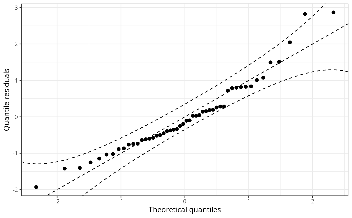
## speed and stopping distances of cars
m1_lm <- lm(dist ~ speed, data = cars)

## compute and plot qqrplot
qqrplot(m1_lm)


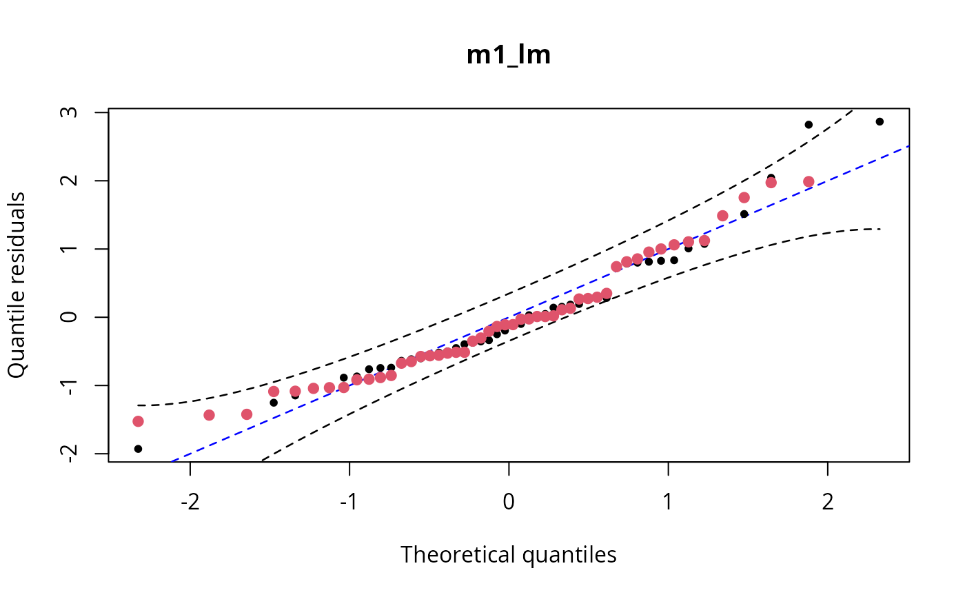
## customize colors
qqrplot(m1_lm, plot = "base", ref_col = "blue", lty = 2, pch = 20)

## add separate model
if (require("crch", quietly = TRUE)) {
  m1_crch <- crch(dist ~ speed | speed, data = cars)
  points(qqrplot(m1_crch, plot = FALSE), col = 2, lty = 2, simint = 2)
}

#> [1] "expected"

#-------------------------------------------------------------------------------
if (require("crch")) {

  ## precipitation observations and forecasts for Innsbruck
  data("RainIbk", package = "crch")
  RainIbk <- sqrt(RainIbk)
  RainIbk$ensmean <- apply(RainIbk[,grep('^rainfc',names(RainIbk))], 1, mean)
  RainIbk$enssd <- apply(RainIbk[,grep('^rainfc',names(RainIbk))], 1, sd)
  RainIbk <- subset(RainIbk, enssd > 0)

  ## linear model w/ constant variance estimation
  m2_lm <- lm(rain ~ ensmean, data = RainIbk)

  ## logistic censored model 
  m2_crch <- crch(rain ~ ensmean | log(enssd), data = RainIbk, left = 0, dist = "logistic")

  ## compute qqrplots
  qq2_lm <- qqrplot(m2_lm, plot = FALSE)
  qq2_crch <- qqrplot(m2_crch, plot = FALSE)

  ## plot in single graph
  plot(c(qq2_lm, qq2_crch), col = c(1, 2), simint_col = c(1, 2), single_graph = TRUE)
}


#-------------------------------------------------------------------------------
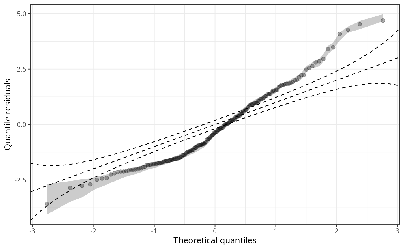
## determinants for male satellites to nesting horseshoe crabs
data("CrabSatellites", package = "countreg")

## linear poisson model
m3_pois  <- glm(satellites ~ width + color, data = CrabSatellites, family = poisson)

## compute and plot qqrplot as "ggplot2" graphic
qqrplot(m3_pois, plot = "ggplot2")

Arguments

Details

References

See also

Examples