S3 Methods for Plotting PIT Histograms
plot.pithist.RdGeneric plotting functions for probability integral transform (PIT)
histograms of the class "pithist" computed by link{pithist}.
# S3 method for pithist
plot(
  x,
  single_graph = FALSE,
  style = NULL,
  freq = NULL,
  expected = TRUE,
  confint = NULL,
  confint_level = 0.95,
  confint_type = c("exact", "approximation"),
  simint = NULL,
  xlim = c(NA, NA),
  ylim = c(0, NA),
  xlab = NULL,
  ylab = NULL,
  main = NULL,
  axes = TRUE,
  box = TRUE,
  col = "black",
  border = "black",
  lwd = NULL,
  lty = 1,
  alpha_min = 0.2,
  expected_col = NULL,
  expected_lty = NULL,
  expected_lwd = 1.75,
  confint_col = NULL,
  confint_lty = 2,
  confint_lwd = 1.75,
  confint_alpha = NULL,
  simint_col = "black",
  simint_lty = 1,
  simint_lwd = 1.75,
  ...
)

# S3 method for pithist
lines(
  x,
  freq = NULL,
  expected = FALSE,
  confint = FALSE,
  confint_level = 0.95,
  confint_type = c("exact", "approximation"),
  simint = FALSE,
  col = "black",
  lwd = 2,
  lty = 1,
  expected_col = "black",
  expected_lty = 2,
  expected_lwd = 1.75,
  confint_col = "black",
  confint_lty = 1,
  confint_lwd = 1.75,
  confint_alpha = 1,
  simint_col = "black",
  simint_lty = 1,
  simint_lwd = 1.75,
  ...
)

# S3 method for pithist
autoplot(
  object,
  single_graph = FALSE,
  style = NULL,
  freq = NULL,
  expected = NULL,
  confint = NULL,
  confint_level = 0.95,
  confint_type = c("exact", "approximation"),
  simint = NULL,
  xlim = c(NA, NA),
  ylim = c(0, NA),
  xlab = NULL,
  ylab = NULL,
  main = NULL,
  legend = FALSE,
  theme = NULL,
  colour = NULL,
  fill = NULL,
  size = NULL,
  linetype = NULL,
  alpha = NULL,
  expected_colour = NULL,
  expected_size = 0.75,
  expected_linetype = NULL,
  expected_alpha = NA,
  confint_colour = NULL,
  confint_fill = NULL,
  confint_size = 0.75,
  confint_linetype = NULL,
  confint_alpha = NULL,
  simint_colour = "black",
  simint_size = 0.5,
  simint_linetype = 1,
  simint_alpha = NA,
  ...
)
Arguments
- single_graph
logical. Should all computed extended reliability diagrams be plotted in a single graph? If yes,
stylemust be set to"line".- style
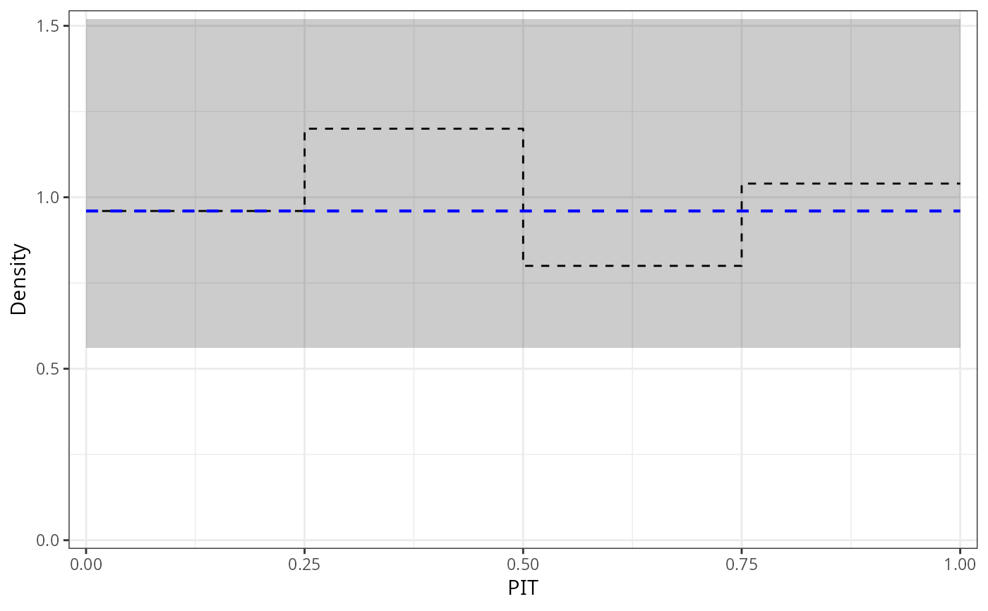
NULLor character specifying the style of pithist. Forstyle = "bar"a traditional PIT hisogram is drawn, forstyle = "line"solely the upper border line is plotted.single_graph = TRUEalways results in a combined line-style PIT histogram.- freq
NULLor logical.TRUEwill enforce the PIT to be represented by frequencies (counts) whileFALSEwill enforce densities.- expected
logical. Should the expected values be plotted as reference?
- confint
NULLor logical. Should confident intervals be drawn? Either logical or as- confint_level
numeric in
[0, 1]. The confidence level to be shown.- confint_type
character. Which type of confidence interval should be plotted: `"exact"` or `"approximation"`. According to Agresti and Coull (1998), for interval estimation of binomial proportions an approximation can be better than exact.
- simint
NULLor logical. In case of discrete distributions, should the simulation (confidence) interval due to the randomization be visualized? character string defining one of `"polygon"`, `"line"` or `"none"`. Iffreq = NULLit is taken from theobject.- xlim, ylim, xlab, ylab, main, axes, box
graphical parameters.
- col, border, lwd, lty, alpha_min
graphical parameters for the main part of the base plot.
- simint_col, simint_lty, simint_lwd, confint_col, confint_lty, confint_lwd, confint_alpha, expected_col, expected_lty, expected_lwd
Further graphical parameters for the `confint` and `simint` line/polygon in the base plot.
- ...
further graphical parameters passed to the plotting function.
- object, x
an object of class
pithist.- legend
logical. Should a legend be added in the
ggplot2style graphic?- theme
Which `ggplot2` theme should be used. If not set,
theme_bwis employed.- colour, fill, size, linetype, alpha
graphical parameters for the histogram style part in the
autoplot.- simint_colour, simint_size, simint_linetype, simint_alpha, confint_colour, confint_fill, confint_size, confint_linetype, expected_colour, expected_size, expected_linetype, expected_alpha
Further graphical parameters for the `confint` and `simint` line/polygon using
autoplot.
Details
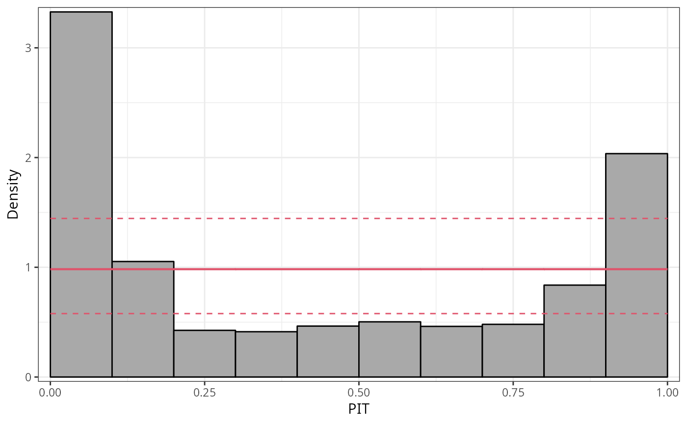
PIT histograms graphically evaluate the probability integral transform (PIT), i.e., the value that the predictive CDF attains at the observation, with a uniform distribution. For a well calibrated model fit, the observation will be drawn from the predictive distribution and the PIT will have a standard uniform distribution.
PIT histograms can be rendered as ggplot2 or base R graphics by using
the generics autoplot or plot.
For a single base R graphically panel, lines adds an additional PIT histogram.
References
Agresti A, Coull AB (1998). “Approximate is Better than ``Exact'' for Interval Estimation of Binomial Proportions.” The American Statistician, 52(2), 119--126. doi:10.1080/00031305.1998.10480550
Czado C, Gneiting T, Held L (2009). “Predictive Model Assessment for Count Data.” Biometrics, 65(4), 1254--1261. doi:10.2307/2981683
Dawid AP (1984). “Present Position and Potential Developments: Some Personal Views: Statistical Theory: The Prequential Approach”, Journal of the Royal Statistical Society: Series A (General), 147(2), 278--292. doi:10.2307/2981683
Diebold FX, Gunther TA, Tay AS (1998). “Evaluating Density Forecasts with Applications to Financial Risk Management”. International Economic Review, 39(4), 863--883. doi:10.2307/2527342
Gneiting T, Balabdaoui F, Raftery AE (2007). “Probabilistic Forecasts, Calibration and Sharpness”. Journal of the Royal Statistical Society: Series B (Methodological). 69(2), 243--268. doi:10.1111/j.1467-9868.2007.00587.x
Examples
## speed and stopping distances of cars
m1_lm <- lm(dist ~ speed, data = cars)
## compute and plot pithist
pithist(m1_lm)
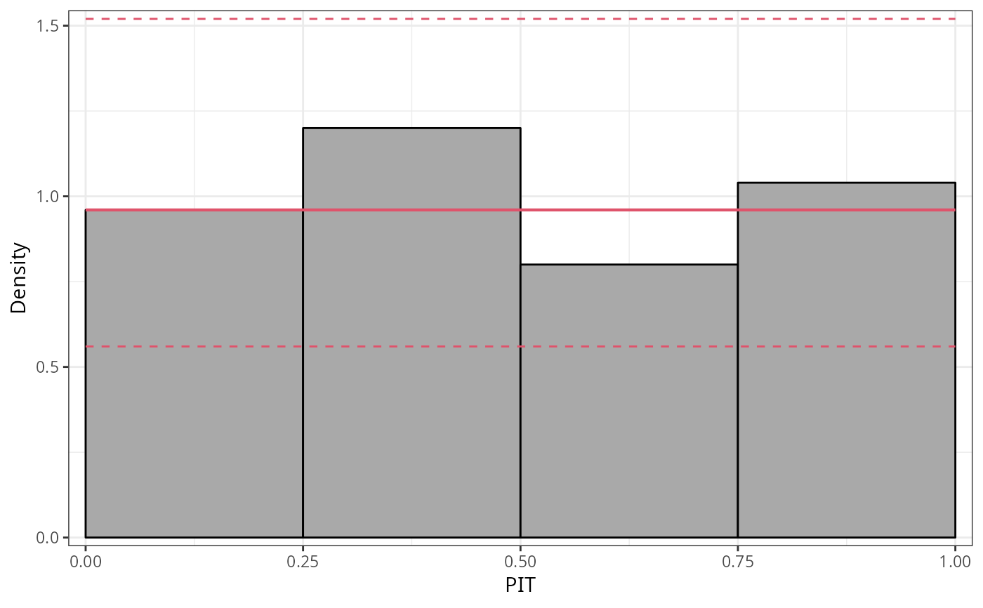 ## customize colors and style
pithist(m1_lm, expected_col = "blue", lty = 2, pch = 20, style = "line")
## customize colors and style
pithist(m1_lm, expected_col = "blue", lty = 2, pch = 20, style = "line")
 ## add separate model
if (require("crch", quietly = TRUE)) {
m1_crch <- crch(dist ~ speed | speed, data = cars)
#lines(pithist(m1_crch, plot = FALSE), col = 2, lty = 2, confint_col = 2) #FIXME
}
#-------------------------------------------------------------------------------
if (require("crch")) {
## precipitation observations and forecasts for Innsbruck
data("RainIbk", package = "crch")
RainIbk <- sqrt(RainIbk)
RainIbk$ensmean <- apply(RainIbk[, grep("^rainfc", names(RainIbk))], 1, mean)
RainIbk$enssd <- apply(RainIbk[, grep("^rainfc", names(RainIbk))], 1, sd)
RainIbk <- subset(RainIbk, enssd > 0)
## linear model w/ constant variance estimation
m2_lm <- lm(rain ~ ensmean, data = RainIbk)
## logistic censored model
m2_crch <- crch(rain ~ ensmean | log(enssd), data = RainIbk, left = 0, dist = "logistic")
## compute pithists
pit2_lm <- pithist(m2_lm, plot = FALSE)
pit2_crch <- pithist(m2_crch, plot = FALSE)
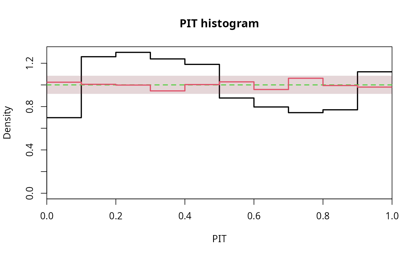
## plot in single graph with style "line"
plot(c(pit2_lm, pit2_crch),
col = c(1, 2), confint_col = c(1, 2), expected_col = 3,
style = "line", single_graph = TRUE
)
}
## add separate model
if (require("crch", quietly = TRUE)) {
m1_crch <- crch(dist ~ speed | speed, data = cars)
#lines(pithist(m1_crch, plot = FALSE), col = 2, lty = 2, confint_col = 2) #FIXME
}
#-------------------------------------------------------------------------------
if (require("crch")) {
## precipitation observations and forecasts for Innsbruck
data("RainIbk", package = "crch")
RainIbk <- sqrt(RainIbk)
RainIbk$ensmean <- apply(RainIbk[, grep("^rainfc", names(RainIbk))], 1, mean)
RainIbk$enssd <- apply(RainIbk[, grep("^rainfc", names(RainIbk))], 1, sd)
RainIbk <- subset(RainIbk, enssd > 0)
## linear model w/ constant variance estimation
m2_lm <- lm(rain ~ ensmean, data = RainIbk)
## logistic censored model
m2_crch <- crch(rain ~ ensmean | log(enssd), data = RainIbk, left = 0, dist = "logistic")
## compute pithists
pit2_lm <- pithist(m2_lm, plot = FALSE)
pit2_crch <- pithist(m2_crch, plot = FALSE)
## plot in single graph with style "line"
plot(c(pit2_lm, pit2_crch),
col = c(1, 2), confint_col = c(1, 2), expected_col = 3,
style = "line", single_graph = TRUE
)
}
 #-------------------------------------------------------------------------------
## determinants for male satellites to nesting horseshoe crabs
data("CrabSatellites", package = "countreg")
## linear poisson model
m3_pois <- glm(satellites ~ width + color, data = CrabSatellites, family = poisson)
## compute and plot pithist as "ggplot2" graphic
pithist(m3_pois, plot = "ggplot2")
#-------------------------------------------------------------------------------
## determinants for male satellites to nesting horseshoe crabs
data("CrabSatellites", package = "countreg")
## linear poisson model
m3_pois <- glm(satellites ~ width + color, data = CrabSatellites, family = poisson)
## compute and plot pithist as "ggplot2" graphic
pithist(m3_pois, plot = "ggplot2")