geom_* and stat_* for Producing Quantile Residual Q-Q Plots with `ggplot2`

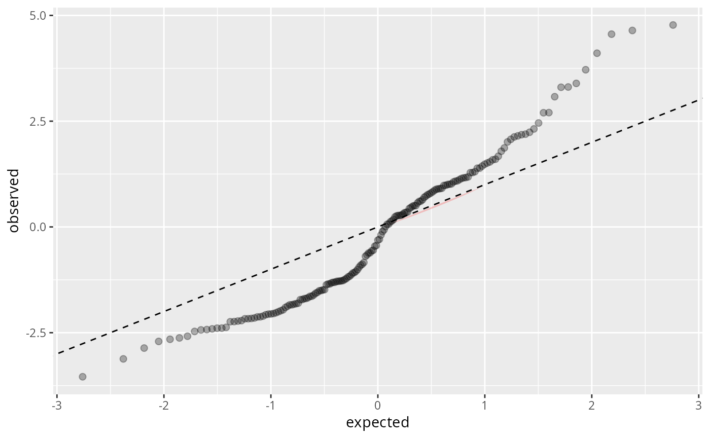
Various geom_* and stat_* used within autoplot for producing quantile residual Q-Q plots.

geom_qqrplot(
  mapping = NULL,
  data = NULL,
  stat = "identity",
  position = "identity",
  na.rm = FALSE,
  show.legend = NA,
  inherit.aes = TRUE,
  ...
)

stat_qqrplot_simint(
  mapping = NULL,
  data = NULL,
  geom = "qqrplot_simint",
  position = "identity",
  na.rm = FALSE,
  show.legend = NA,
  inherit.aes = TRUE,
  ...
)

geom_qqrplot_simint(
  mapping = NULL,
  data = NULL,
  stat = "qqrplot_simint",
  position = "identity",
  na.rm = FALSE,
  show.legend = NA,
  inherit.aes = TRUE,
  ...
)

stat_qqrplot_ref(
  mapping = NULL,
  data = NULL,
  geom = "qqrplot_ref",
  position = "identity",
  na.rm = FALSE,
  show.legend = NA,
  inherit.aes = TRUE,
  detrend = FALSE,
  identity = TRUE,
  probs = c(0.25, 0.75),
  scale = c("normal", "uniform"),
  ...
)

geom_qqrplot_ref(
  mapping = NULL,
  data = NULL,
  stat = "qqrplot_ref",
  position = "identity",
  na.rm = FALSE,
  show.legend = NA,
  inherit.aes = TRUE,
  detrend = FALSE,
  identity = TRUE,
  probs = c(0.25, 0.75),
  scale = c("normal", "uniform"),
  ...
)

geom_qqrplot_confint(
  mapping = NULL,
  data = NULL,
  stat = "qqrplot_confint",
  position = "identity",
  na.rm = FALSE,
  show.legend = NA,
  inherit.aes = TRUE,
  xlim = NULL,
  n = 101,
  detrend = FALSE,
  type = c("pointwise", "simultaneous", "tail-sensitive"),
  level = 0.95,
  identity = TRUE,
  probs = c(0.25, 0.75),
  scale = c("normal", "uniform"),
  style = c("polygon", "line"),
  ...
)

GeomQqrplotConfint

Format

An object of class GeomQqrplotConfint (inherits from Geom, ggproto, gg) of length 6.

Arguments

mapping

Set of aesthetic mappings created by aes(). If specified and inherit.aes = TRUE (the default), it is combined with the default mapping at the top level of the plot. You must supply mapping if there is no plot mapping.

data

The data to be displayed in this layer. There are three options:

If NULL, the default, the data is inherited from the plot data as specified in the call to ggplot().

A data.frame, or other object, will override the plot data. All objects will be fortified to produce a data frame. See fortify() for which variables will be created.

A function will be called with a single argument, the plot data. The return value must be a data.frame, and will be used as the layer data. A function can be created from a formula (e.g. ~ head(.x, 10)).

stat

The statistical transformation to use on the data for this layer, either as a ggproto Geom subclass or as a string naming the stat stripped of the stat_ prefix (e.g. "count" rather than "stat_count")

position

Position adjustment, either as a string naming the adjustment (e.g. "jitter" to use position_jitter), or the result of a call to a position adjustment function. Use the latter if you need to change the settings of the adjustment.

na.rm

If FALSE, the default, missing values are removed with a warning. If TRUE, missing values are silently removed.

show.legend

logical. Should this layer be included in the legends? NA, the default, includes if any aesthetics are mapped. FALSE never includes, and TRUE always includes. It can also be a named logical vector to finely select the aesthetics to display.

inherit.aes

If FALSE, overrides the default aesthetics, rather than combining with them. This is most useful for helper functions that define both data and aesthetics and shouldn't inherit behaviour from the default plot specification, e.g. borders().

...

Other arguments passed on to layer(). These are often aesthetics, used to set an aesthetic to a fixed value, like colour = "red" or size = 3. They may also be parameters to the paired geom/stat.

geom

The geometric object to use to display the data, either as a ggproto Geom subclass or as a string naming the geom stripped of the geom_ prefix (e.g. "point" rather than "geom_point")

detrend

logical, default FALSE. If set to TRUE the qqrplot is detrended, i.e, plotted as a wormplot.

identity

logical. Should the identity line be plotted or a theoretical line which passes through probs quantiles on the "uniform" or "normal" scale.

probs

numeric vector of length two, representing probabilities of reference line used.

scale

character. Scale on which the quantile residuals will be shown: "uniform" (default) for uniform scale or "normal" for normal scale. Used for the reference line which goes through the first and third quartile of theoretical distributions.

xlim

NULL (default) or numeric. The x limits for computing the confidence intervals.

n

positive numeric. Number of points used to compute the confidence intervals, the more the smoother.

type

character. Should "pointwise" (default), "simultaneous", or "tail-sensitive" confidence intervals of the (randomized) quantile residuals be visualized. Simultaneous confidence intervals are based on the Kolmogorov-Smirnov test.

level

numeric. The confidence level required, defaults to 0.95.

style

character. Style for plotting confidence intervals. Either "polygon" (default) or "line").

Examples

if (require("ggplot2")) {
  ## Fit model
  data("CrabSatellites", package = "countreg")
  m1_pois <- glm(satellites ~ width + color, data = CrabSatellites, family = poisson)
  m2_pois <- glm(satellites ~ color, data = CrabSatellites, family = poisson)
  
  ## Compute qqrplot
  q1 <- qqrplot(m1_pois, plot = FALSE)
  q2 <- qqrplot(m2_pois, plot = FALSE)
  
  d <- c(q1, q2) 
  
  ## Get label names
  xlab <- unique(attr(d, "xlab"))
  ylab <- unique(attr(d, "ylab"))
  main <- attr(d, "main")
  main <- make.names(main, unique = TRUE)
  d$group <- factor(d$group, labels = main)
  
  ## Polygon CI around identity line used as reference 
  gg1 <- ggplot(data = d, aes(x = expected, y = observed, na.rm = TRUE)) + 
    geom_qqrplot_ref() + 
    geom_qqrplot_confint(fill = "red") + 
    geom_qqrplot() + 
    geom_qqrplot_simint(
      aes(
        x = simint_expected, 
        ymin = simint_observed_lwr, 
        ymax = simint_observed_upr,
        group = group
      )
    ) + 
    xlab(xlab) + ylab(ylab)

  gg1
  gg1 + facet_wrap(~group)
  
  ## Polygon CI around robust reference line
  gg2 <- ggplot(data = d, aes(x = expected, y = observed, na.rm = TRUE)) + 
    geom_qqrplot_ref(identity = FALSE, scale = attr(d, "scale")) + 
    geom_qqrplot_confint(identity = FALSE, scale = attr(d, "scale"), style = "line") + 
    geom_qqrplot() + 
    geom_qqrplot_simint(
      aes(
        x = simint_expected, 
        ymin = simint_observed_lwr, 
        ymax = simint_observed_upr,
        group = group
      )
    ) + 
    xlab(xlab) + ylab(ylab)

  gg2
  gg2 + facet_wrap(~group)

  ## Use different `scale`s with confidence intervals
  q1 <- qqrplot(m1_pois, scale = "uniform", plot = FALSE)
  q2 <- qqrplot(m2_pois, plot = FALSE)
  
  gg3 <- ggplot(data = q1, aes(x = expected, y = observed, na.rm = TRUE)) +
    geom_qqrplot_ref() +
    geom_qqrplot_confint(fill = "red", scale = "uniform") +
    geom_qqrplot()
  gg3
  
  gg4 <- ggplot(data = q2, aes(x = expected, y = observed, na.rm = TRUE)) +
    geom_qqrplot_ref() +
    geom_qqrplot_confint(fill = "red", scale = "uniform") +
    geom_qqrplot()
  gg4
} 
#> Warning: Using the `size` aesthetic in this geom was deprecated in ggplot2 3.4.0.
#> ℹ Please use `linewidth` in the `default_aes` field and elsewhere instead.