geom_* and stat_* for Producing PIT Histograms with `ggplot2`

Various geom_* and stat_* used within autoplot for producing PIT histograms.

stat_pithist(
  mapping = NULL,
  data = NULL,
  geom = "pithist",
  position = "identity",
  na.rm = FALSE,
  show.legend = NA,
  inherit.aes = TRUE,
  freq = FALSE,
  style = c("bar", "line"),
  ...
)

geom_pithist(
  mapping = NULL,
  data = NULL,
  stat = "pithist",
  position = "identity",
  na.rm = FALSE,
  show.legend = NA,
  inherit.aes = TRUE,
  freq = FALSE,
  style = c("bar", "line"),
  ...
)

stat_pithist_expected(
  mapping = NULL,
  data = NULL,
  geom = "pithist_expected",
  position = "identity",
  na.rm = FALSE,
  show.legend = NA,
  inherit.aes = TRUE,
  scale = c("uniform", "normal"),
  freq = FALSE,
  ...
)

geom_pithist_expected(
  mapping = NULL,
  data = NULL,
  stat = "pithist_expected",
  position = "identity",
  na.rm = FALSE,
  show.legend = NA,
  inherit.aes = TRUE,
  scale = c("uniform", "normal"),
  freq = FALSE,
  ...
)

stat_pithist_confint(
  mapping = NULL,
  data = NULL,
  geom = "pithist_confint",
  position = "identity",
  na.rm = FALSE,
  show.legend = NA,
  inherit.aes = TRUE,
  scale = c("uniform", "normal"),
  level = 0.95,
  type = "approximation",
  freq = FALSE,
  style = c("polygon", "line"),
  ...
)

geom_pithist_confint(
  mapping = NULL,
  data = NULL,
  stat = "pithist_confint",
  position = "identity",
  na.rm = FALSE,
  show.legend = NA,
  inherit.aes = TRUE,
  scale = c("uniform", "normal"),
  level = 0.95,
  type = "approximation",
  freq = FALSE,
  style = c("polygon", "line"),
  ...
)

stat_pithist_simint(
  mapping = NULL,
  data = NULL,
  geom = "pithist_simint",
  position = "identity",
  na.rm = FALSE,
  show.legend = NA,
  inherit.aes = TRUE,
  freq = FALSE,
  ...
)

geom_pithist_simint(
  mapping = NULL,
  data = NULL,
  stat = "pithist_simint",
  position = "identity",
  na.rm = FALSE,
  show.legend = NA,
  inherit.aes = TRUE,
  freq = FALSE,
  ...
)

Arguments

mapping

Set of aesthetic mappings created by aes(). If specified and inherit.aes = TRUE (the default), it is combined with the default mapping at the top level of the plot. You must supply mapping if there is no plot mapping.

data

The data to be displayed in this layer. There are three options:

If NULL, the default, the data is inherited from the plot data as specified in the call to ggplot().

A data.frame, or other object, will override the plot data. All objects will be fortified to produce a data frame. See fortify() for which variables will be created.

A function will be called with a single argument, the plot data. The return value must be a data.frame, and will be used as the layer data. A function can be created from a formula (e.g. ~ head(.x, 10)).

geom

The geometric object to use to display the data, either as a ggproto Geom subclass or as a string naming the geom stripped of the geom_ prefix (e.g. "point" rather than "geom_point")

position

Position adjustment, either as a string naming the adjustment (e.g. "jitter" to use position_jitter), or the result of a call to a position adjustment function. Use the latter if you need to change the settings of the adjustment.

na.rm

If FALSE, the default, missing values are removed with a warning. If TRUE, missing values are silently removed.

show.legend

logical. Should this layer be included in the legends? NA, the default, includes if any aesthetics are mapped. FALSE never includes, and TRUE always includes. It can also be a named logical vector to finely select the aesthetics to display.

inherit.aes

If FALSE, overrides the default aesthetics, rather than combining with them. This is most useful for helper functions that define both data and aesthetics and shouldn't inherit behaviour from the default plot specification, e.g. borders().

freq

logical. If TRUE, the PIT histogram is represented by frequencies, the counts component of the result; if FALSE, probability densities, component density, are plotted (so that the histogram has a total area of one).

style

character specifying the style of pithist. For style = "bar" a traditional PIT hisogram is drawn, for style = "line" solely the upper border line is plotted.

...

Other arguments passed on to layer(). These are often aesthetics, used to set an aesthetic to a fixed value, like colour = "red" or size = 3. They may also be parameters to the paired geom/stat.

stat

The statistical transformation to use on the data for this layer, either as a ggproto Geom subclass or as a string naming the stat stripped of the stat_ prefix (e.g. "count" rather than "stat_count")

scale

On which scale should the PIT residuals be computed: on the probability scale ("uniform") or on the normal scale ("normal").

level

numeric. The confidence level required.

type

character. Which type of confidence interval should be plotted: `"exact"` or `"approximation"`. According to Agresti and Coull (1998), for interval estimation of binomial proportions an approximation can be better than exact.

Examples

if (require("ggplot2")) {
  ## Fit model
  data("CrabSatellites", package = "countreg")
  m1_pois <- glm(satellites ~ width + color, data = CrabSatellites, family = poisson)
  m2_pois <- glm(satellites ~ color, data = CrabSatellites, family = poisson)

  ## Compute pithist
  p1 <- pithist(m1_pois, type = "random", plot = FALSE)
  p2 <- pithist(m2_pois, type = "random", plot = FALSE)

  d <- c(p1, p2)

  ## Create factor
  main <- attr(d, "main")
  main <- make.names(main, unique = TRUE)
  d$group <- factor(d$group, labels = main)

  ## Plot bar style PIT histogram
  gg1 <- ggplot(data = d) +
    geom_pithist(aes(x = mid, y = observed, width = width, group = group), freq = TRUE) +
    geom_pithist_simint(aes(x = mid, ymin = simint_lwr, ymax = simint_upr), freq = TRUE) +
    geom_pithist_confint(aes(x = mid, y = observed, width = width), style = "line", freq = TRUE) +
    geom_pithist_expected(aes(x = mid, y = observed, width = width), freq = TRUE) +
    facet_grid(group ~ .) +
    xlab("PIT") +
    ylab("Frequency")
  gg1

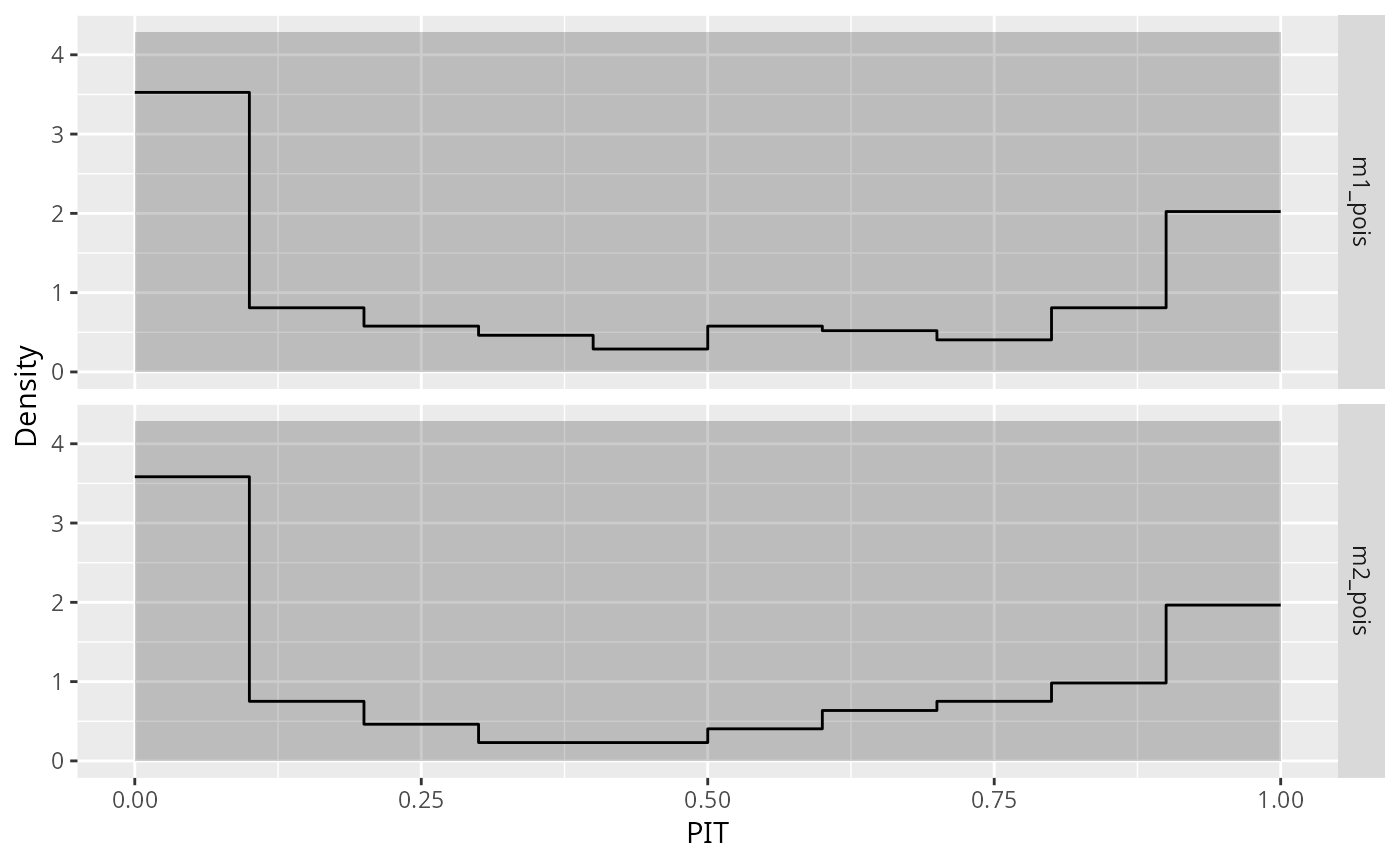
  gg2 <- ggplot(data = d) +
    geom_pithist(aes(x = mid, y = observed, width = width, group = group), freq = FALSE) +
    geom_pithist_simint(aes(
      x = mid, ymin = simint_lwr, ymax = simint_upr, y = observed,
      width = width
    ), freq = FALSE) +
    geom_pithist_confint(aes(x = mid, y = observed, width = width), style = "line", freq = FALSE) +
    geom_pithist_expected(aes(x = mid, y = observed, width = width), freq = FALSE) +
    facet_grid(group ~ .) +
    xlab("PIT") +
    ylab("Density")
  gg2

  ## Plot line style PIT histogram
  gg3 <- ggplot(data = d) +
    geom_pithist(aes(x = mid, y = observed, width = width, group = group), style = "line") +
    geom_pithist_confint(aes(x = mid, y = observed, width = width), style = "polygon") +
    facet_grid(group ~ .) +
    xlab("PIT") +
    ylab("Density")
  gg3
}
#> Loading required package: ggplot2