Create a GAMLSS Distribution

A single class and corresponding methods encompassing all distributions from the gamlss.dist package using the workflow from the distributions3 package.

GAMLSS(family, mu, sigma, tau, nu)

Arguments

family: character. Name of a GAMLSS family provided by gamlss.dist, e.g., NO or BI for the normal or binomial distribution, respectively.
mu: numeric. GAMLSS mu parameter. Can be a scalar or a vector or missing if not part of the family.
sigma: numeric. GAMLSS sigma parameter. Can be a scalar or a vector or missing if not part of the family.
tau: numeric. GAMLSS tau parameter. Can be a scalar or a vector or missing if not part of the family.
nu: numeric. GAMLSS nu parameter. Can be a scalar or a vector or missing if not part of the family.

Value

A GAMLSS distribution object.

Details

The constructor function GAMLSS sets up a distribution object, representing a distribution from the GAMLSS (generalized additive model of location, scale, and shape) framework by the corresponding parameters plus a family attribute, e.g., NO for the normal distribution or BI for the binomial distribution. There can be up to four parameters, called mu (often some sort of location parameter), sigma (often some sort of scale parameter), tau and nu (other parameters, e.g., capturing shape, etc.).

All parameters can also be vectors, so that it is possible to define a vector of GAMLSS distributions from the same family with potentially different parameters. All parameters need to have the same length or must be scalars (i.e., of length 1) which are then recycled to the length of the other parameters.

Note that not all distributions use all four parameters, i.e., some use just a subset. In that case, the corresponding arguments in GAMLSS should be unspecified, NULL, or NA.

For the GAMLSS distribution objects there is a wide range of standard methods available to the generics provided in the distributions3 package: pdf and log_pdf for the (log-)density (PDF), cdf for the probability from the cumulative distribution function (CDF), quantile for quantiles, random for simulating random variables, and support for the support interval (minimum and maximum). Internally, these methods rely on the usual d/p/q/r functions provided in gamlss.dist, see the manual pages of the individual families. The methods is_discrete and is_continuous can be used to query whether the distributions are discrete on the entire support or continuous on the entire support, respectively.

Additionally, for some families there is also a crps method for computing the continuous ranked probability score (CRPS) via the scoringRules package. This is only available for those families which are supported by both packages.

See the examples below for an illustration of the workflow for the class and methods.

Examples

 if(!requireNamespace("gamlss.dist")) {
  if(interactive() || is.na(Sys.getenv("_R_CHECK_PACKAGE_NAME_", NA))) {
    stop("not all packages required for the example are installed")
  } else q() }
#> Loading required namespace: gamlss.dist
#> Registered S3 methods overwritten by 'gamlss.dist':
#>   method          from     
#>   format.GAMLSS   topmodels
#>   print.GAMLSS    topmodels
#>   mean.GAMLSS     topmodels
#>   quantile.GAMLSS topmodels

## package and random seed
library("distributions3")
set.seed(6020)

## three Weibull distributions
X <- GAMLSS("WEI", mu = c(1, 1, 2), sigma = c(1, 2, 2))
X
#> [1] "GAMLSS WEI distribution (mu = 1, sigma = 1)"
#> [2] "GAMLSS WEI distribution (mu = 1, sigma = 2)"
#> [3] "GAMLSS WEI distribution (mu = 2, sigma = 2)"

## moments
mean(X)
#> [1] 1.0000000 0.8862269 1.7724539
variance(X)
#> [1] 1.0000000 0.2146018 0.8584073

## support interval (minimum and maximum)
support(X)
#>      min max
#> [1,]   0 Inf
#> [2,]   0 Inf
#> [3,]   0 Inf
is_discrete(X)
#> [1] FALSE FALSE FALSE
is_continuous(X)
#> [1] TRUE TRUE TRUE

## simulate random variables
random(X, 5)
#>           r_1       r_2       r_3      r_4      r_5
#> [1,] 1.004812 0.3993868 1.3084904 0.741085 3.209012
#> [2,] 1.023982 0.5593371 0.5440658 1.046042 2.244104
#> [3,] 1.254624 2.8848168 3.0103388 2.166692 2.572731

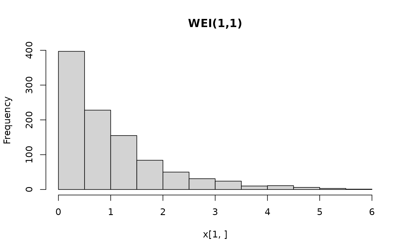
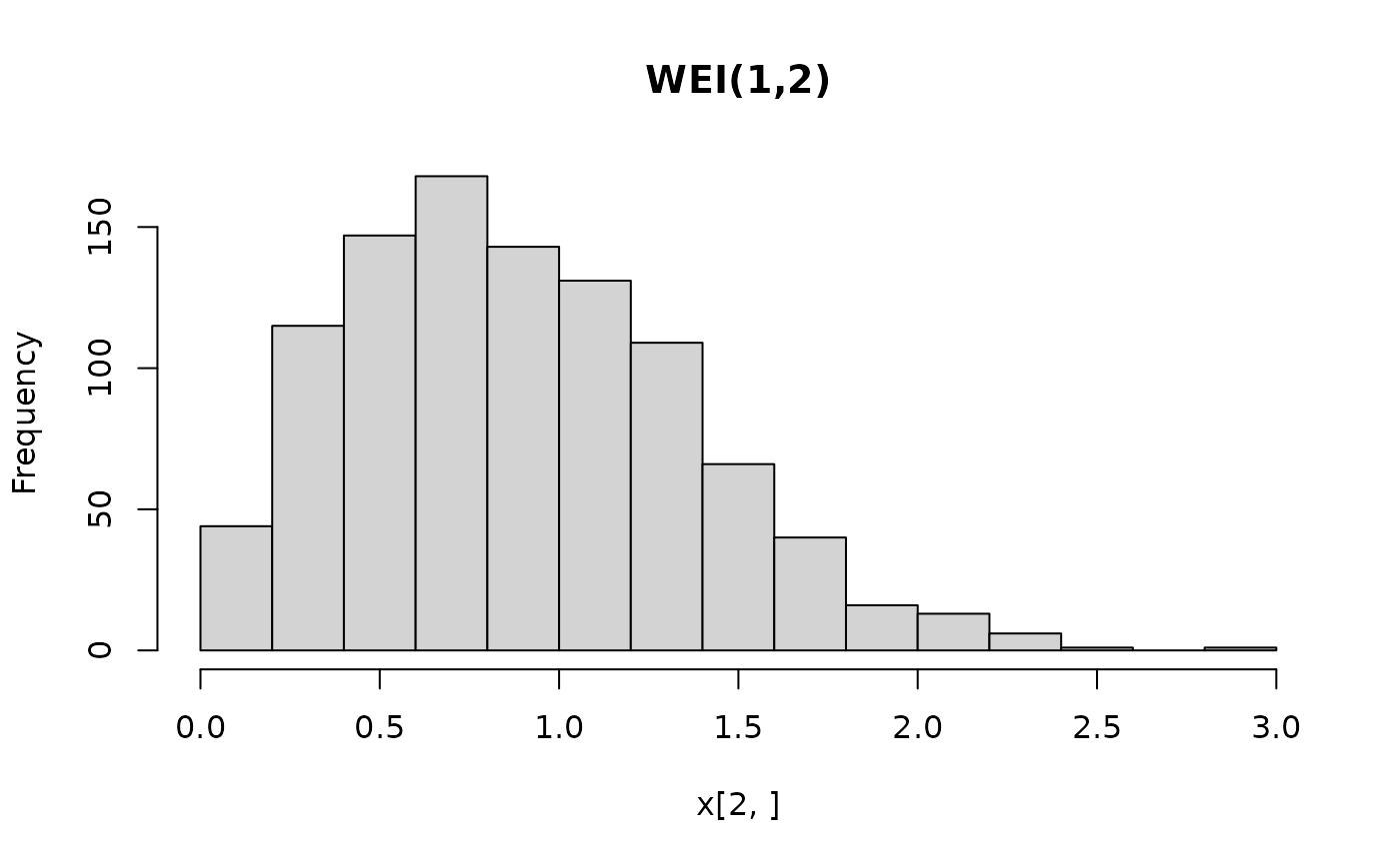
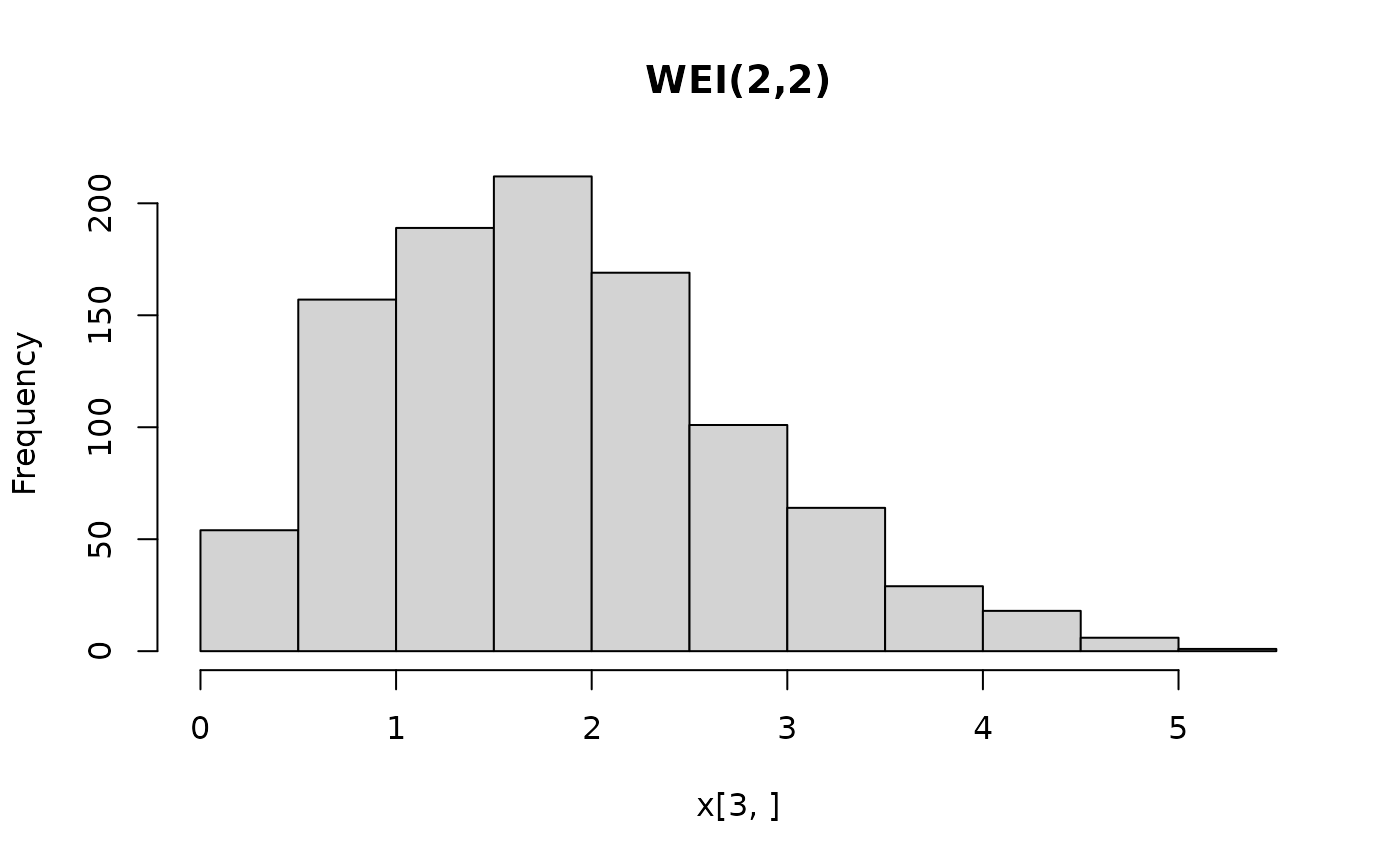
## histograms of 1,000 simulated observations
x <- random(X, 1000)
hist(x[1, ], main = "WEI(1,1)")

hist(x[2, ], main = "WEI(1,2)")

hist(x[3, ], main = "WEI(2,2)")


## probability density function (PDF) and log-density (or log-likelihood)
x <- c(2, 2, 1)
pdf(X, x)
#> [1] 0.13533528 0.07326256 0.38940039
pdf(X, x, log = TRUE)
#> [1] -2.0000000 -2.6137056 -0.9431472
log_pdf(X, x)
#> [1] -2.0000000 -2.6137056 -0.9431472

## cumulative distribution function (CDF)
cdf(X, x)
#> [1] 0.8646647 0.9816844 0.2211992

## quantiles
quantile(X, 0.5)
#> [1] 0.6931472 0.8325546 1.6651092

## cdf() and quantile() are inverses
cdf(X, quantile(X, 0.5))
#> [1] 0.5 0.5 0.5
quantile(X, cdf(X, 1))
#> [1] 1 1 1

## all methods above can either be applied elementwise or for
## all combinations of X and x, if length(X) = length(x),
## also the result can be assured to be a matrix via drop = FALSE
p <- c(0.05, 0.5, 0.95)
quantile(X, p, elementwise = FALSE)
#>          q_0.05     q_0.5   q_0.95
#> [1,] 0.05129329 0.6931472 2.995732
#> [2,] 0.22648023 0.8325546 1.730818
#> [3,] 0.45296046 1.6651092 3.461637
quantile(X, p, elementwise = TRUE)
#> [1] 0.05129329 0.83255461 3.46163677
quantile(X, p, elementwise = TRUE, drop = FALSE)
#>        quantile
#> [1,] 0.05129329
#> [2,] 0.83255461
#> [3,] 3.46163677

## compare theoretical and empirical mean from 1,000 simulated observations
cbind(
  "theoretical" = mean(X),
  "empirical" = rowMeans(random(X, 1000))
)
#>      theoretical empirical
#> [1,]   1.0000000 1.0075953
#> [2,]   0.8862269 0.9057806
#> [3,]   1.7724539 1.7587308

Arguments

Value

Details

See also

Examples