S3 Methods for a Reliagram (Extended Reliability Diagram)

Generic plotting functions for reliability diagrams of the class "reliagram" computed by link{reliagram}.

# S3 method for reliagram
plot(
  x,
  single_graph = FALSE,
  minimum = 0,
  confint = TRUE,
  ref = TRUE,
  xlim = c(0, 1),
  ylim = c(0, 1),
  xlab = NULL,
  ylab = NULL,
  main = NULL,
  col = "black",
  fill = adjustcolor("black", alpha.f = 0.2),
  alpha_min = 0.2,
  lwd = 2,
  pch = 19,
  lty = 1,
  type = NULL,
  add_hist = TRUE,
  add_info = TRUE,
  add_rug = TRUE,
  add_min = TRUE,
  axes = TRUE,
  box = TRUE,
  ...
)

# S3 method for reliagram
lines(
  x,
  minimum = 0,
  confint = FALSE,
  ref = FALSE,
  col = "black",
  fill = adjustcolor("black", alpha.f = 0.2),
  alpha_min = 0.2,
  lwd = 2,
  pch = 19,
  lty = 1,
  type = "b",
  ...
)

# S3 method for reliagram
autoplot(
  object,
  single_graph = FALSE,
  minimum = 0,
  confint = TRUE,
  ref = TRUE,
  xlim = c(0, 1),
  ylim = c(0, 1),
  xlab = NULL,
  ylab = NULL,
  main = NULL,
  colour = "black",
  fill = adjustcolor("black", alpha.f = 0.2),
  alpha_min = 0.2,
  size = 1,
  shape = 19,
  linetype = 1,
  type = NULL,
  add_hist = TRUE,
  add_info = TRUE,
  add_rug = TRUE,
  add_min = TRUE,
  legend = FALSE,
  ...
)

Arguments

single_graph

logical. Should all computed extended reliability diagrams be plotted in a single graph?

minimum, ref, xlim, ylim, col, fill, alpha_min, lwd, pch, lty, type, add_hist, add_info, add_rug, add_min, axes, box

additional graphical parameters for base plots, whereby x is a object of class reliagram.

confint

logical. Should confident intervals be calculated and drawn?

xlab, ylab, main

graphical parameters.

...

further graphical parameters.

object, x

an object of class reliagram.

colour, size, shape, linetype, legend

graphical parameters passed for ggplot2 style plots, whereby object is a object of class reliagram.

Details

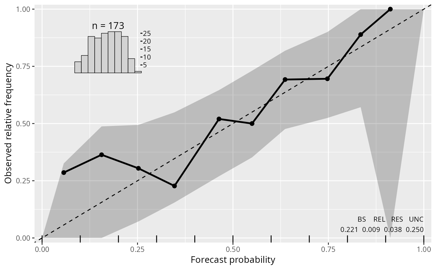
Reliagrams evaluate if a probability model is calibrated (reliable) by first partitioning the forecast probability for a binary event into a certain number of bins and then plotting (within each bin) the averaged forecast probability against the observered/empirical relative frequency.

For continous probability forecasts, reliability diagrams can be plotted either for a pre-specified threshold or for a specific quantile probability of the response values.

Reliagrams can be rendered as ggplot2 or base R graphics by using the generics autoplot or plot. For a single base R graphically panel, points adds an additional reliagram.

References

Wilks DS (2011) Statistical Methods in the Atmospheric Sciences, 3rd ed., Academic Press, 704 pp.

See also

link{reliagram}, procast

Examples

## speed and stopping distances of cars
m1_lm <- lm(dist ~ speed, data = cars)

## compute and plot reliagram
reliagram(m1_lm)


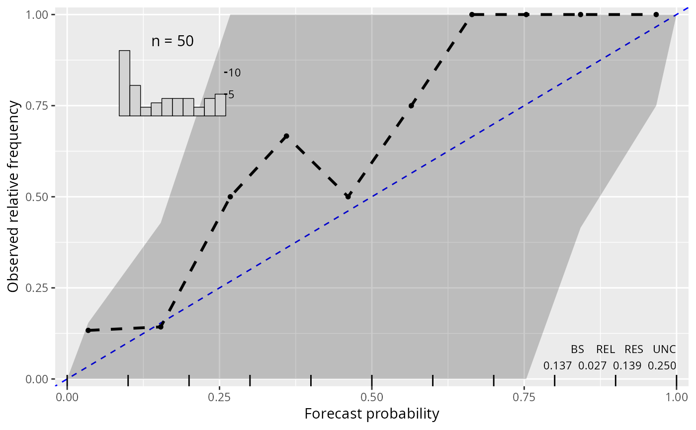
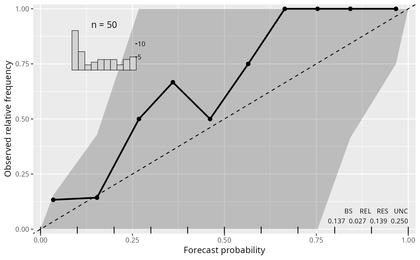## customize colors
reliagram(m1_lm, ref = "blue", lty = 2, pch = 20)


## add separate model
if (require("crch", quietly = TRUE)) {
  m1_crch <- crch(dist ~ speed | speed, data = cars)
  lines(reliagram(m1_crch, plot = FALSE), col = 2, lty = 2, confint = 2)
}
#> Error in polygon(na.omit(c(ifelse(extend_left, 0, NA), d[min_idx, "x"],     ifelse(extend_right, 1, NA), rev(d[min_idx, "x"]), ifelse(extend_left,         0, NA))), na.omit(c(ifelse(extend_left, 0, NA), d[min_idx,     "ci_lwr"], ifelse(extend_right, 1, NA), rev(d[min_idx, "ci_upr"]),     ifelse(extend_left, 0, NA))), col = set_minimum_transparency(plot_arg$confint[j],     alpha_min = plot_arg$alpha_min[j]), border = NA): plot.new has not been called yet

#-------------------------------------------------------------------------------
if (require("crch")) {

  ## precipitation observations and forecasts for Innsbruck
  data("RainIbk", package = "crch")
  RainIbk <- sqrt(RainIbk)
  RainIbk$ensmean <- apply(RainIbk[,grep('^rainfc',names(RainIbk))], 1, mean)
  RainIbk$enssd <- apply(RainIbk[,grep('^rainfc',names(RainIbk))], 1, sd)
  RainIbk <- subset(RainIbk, enssd > 0)

  ## linear model w/ constant variance estimation
  m2_lm <- lm(rain ~ ensmean, data = RainIbk)

  ## logistic censored model 
  m2_crch <- crch(rain ~ ensmean | log(enssd), data = RainIbk, left = 0, dist = "logistic")

  ## compute reliagrams
  rel2_lm <- reliagram(m2_lm, plot = FALSE)
  rel2_crch <- reliagram(m2_crch, plot = FALSE)

  ## plot in single graph
  plot(c(rel2_lm, rel2_crch), col = c(1, 2), confint = c(1, 2), ref = 3, single_graph = TRUE)
}

#-------------------------------------------------------------------------------
## determinants for male satellites to nesting horseshoe crabs
data("CrabSatellites", package = "countreg")

## linear poisson model
m3_pois  <- glm(satellites ~ width + color, data = CrabSatellites, family = poisson)

## compute and plot reliagram as "ggplot2" graphic
reliagram(m3_pois, plot = "ggplot2")